I’ve spent so many years using and broadcasting my love for R and using Python quite minimally. Having read recently about machine learning in Python, I decided to take on a fun little ML project using Python from start to finish.

What follows below takes advantage of a neat dataset from the UCI Machine Learning Repository.  The data contain Math test performance of 649 students in 2 Portuguese schools.  What’s neat about this data set is that in addition to grades on the students’ 3 Math tests, they managed to collect a whole whack of demographic variables (and some behavioural) as well.  That lead me to the question of how well can you predict final math test performance based on demographics and behaviour alone.  In other words, who is likely to do well, and who is likely to tank?

I have to admit before I continue, I initially intended on doing this analysis in Python alone, but I actually felt lost 3 quarters of the way through and just did the whole darned thing in R.  Once I had completed the analysis in R to my liking, I then went back to my Python analysis and continued until I finished to my reasonable satisfaction.  For that reason, for each step in the analysis, I will show you the code I used in Python, the results, and then the same thing in R.  Do not treat this as a comparison of Python’s machine learning capabilities versus R per se.  Please treat this as a comparison of my understanding of how to do machine learning in Python versus R!

Without further ado, let’s start with some import statements in Python and library statements in R:

#Python Code
from pandas import *
from matplotlib import *
import seaborn as sns
sns.set_style("darkgrid")
import matplotlib.pyplot as plt
%matplotlib inline # I did this in ipython notebook, this makes the graphs show up inline in the notebook.
import statsmodels.formula.api as smf
from scipy import stats
from numpy.random import uniform
from numpy import arange
from sklearn.ensemble import RandomForestRegressor
from sklearn.metrics import mean_squared_error
from math import sqrt
mat_perf = read_csv('/home/inkhorn/Student Performance/student-mat.csv', delimiter=';')

I’d like to comment on the number of import statements I found myself writing in this python script. Eleven!! Is that even normal? Note the smaller number of library statements in my R code block below:

#R Code
library(ggplot2)
library(dplyr)
library(ggthemr)
library(caret)
ggthemr('flat') # I love ggthemr!
mat_perf = read.csv('student-mat.csv', sep = ';')

Now let’s do a quick plot of our target variable, scores on the students’ final math test, named ‘G3′.

#Python Code
sns.set_palette("deep", desat=.6)
sns.set_context(context='poster', font_scale=1)
sns.set_context(rc={"figure.figsize": (8, 4)})
plt.hist(mat_perf.G3)
plt.xticks(range(0,22,2))

Distribution of Final Math Test Scores (“G3″)

That looks pretty pleasing to my eyes. Now let’s see the code for the same thing in R (I know, the visual theme is different. So sue me!)

#R Code
ggplot(mat_perf) + geom_histogram(aes(x=G3), binwidth=2)

You’ll notice that I didn’t need to tweak any palette or font size parameters for the R plot, because I used the very fun ggthemr package. You choose the visual theme you want, declare it early on, and then all subsequent plots will share the same theme! There is a command I’ve hidden, however, modifying the figure height and width. I set the figure size using rmarkdown, otherwise I just would have sized it manually using the export menu in the plot frame in RStudio.  I think both plots look pretty nice, although I’m very partial to working with ggthemr!

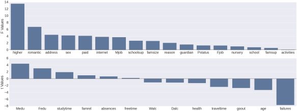
Univariate estimates of variable importance for feature selection

Below, what I’ve done in both languages is to cycle through each variable in the dataset (excepting prior test scores) insert the variable name in a dictionary/list, and get a measure of importance of how predictive that variable is, alone, of the final math test score (variable G3). Of course if the variable is qualitative then I get an F score from an ANOVA, and if it’s quantitative then I get a t score from the regression.

In the case of Python this is achieved in both cases using the ols function from scipy’s statsmodels package. In the case of R I’ve achieved this using the aov function for qualitative and the lm function for quantitative variables. The numerical outcome, as you’ll see from the graphs, is the same.

#Python Code
test_stats = {'variable': [], 'test_type' : [], 'test_value' : []}

for col in mat_perf.columns[:-3]:
    test_stats['variable'].append(col)
    if mat_perf[col].dtype == 'O':
        # Do ANOVA
        aov = smf.ols(formula='G3 ~ C(' + col + ')', data=mat_perf, missing='drop').fit()
        test_stats['test_type'].append('F Test')
        test_stats['test_value'].append(round(aov.fvalue,2))
    else:
        # Do correlation
        print col + 'n'
        model = smf.ols(formula='G3 ~ ' + col, data=mat_perf, missing='drop').fit()
        value = round(model.tvalues[1],2)
        test_stats['test_type'].append('t Test')
        test_stats['test_value'].append(value)

test_stats = DataFrame(test_stats)
test_stats.sort(columns='test_value', ascending=False, inplace=True)

#R Code
test.stats = list(test.type = c(), test.value = c(), variable = c())

for (i in 1:30) {
  test.stats$variable[i] = names(mat_perf)[i]
  if (is.factor(mat_perf[,i])) {
    anova = summary(aov(G3 ~ mat_perf[,i], data=mat_perf))
    test.stats$test.type[i] = "F test"
    test.stats$test.value[i] = unlist(anova)[7]
  }
  else {
    reg = summary(lm(G3 ~ mat_perf[,i], data=mat_perf))
    test.stats$test.type[i] = "t test"
    test.stats$test.value[i] = reg$coefficients[2,3]
  }

}

test.stats.df = arrange(data.frame(test.stats), desc(test.value))
test.stats.df$variable = reorder(test.stats.df$variable, -test.stats.df$test.value)

And now for the graphs. Again you’ll see a bit more code for the Python graph vs the R graph. Perhaps someone will be able to show me code that doesn’t involve as many lines, or maybe it’s just the way things go with graphing in Python. Feel free to educate me :)

#Python Code
f, (ax1, ax2) = plt.subplots(2,1, figsize=(48,18), sharex=False)
sns.set_context(context='poster', font_scale=1)
sns.barplot(x='variable', y='test_value', data=test_stats.query("test_type == 'F Test'"), hline=.1, ax=ax1, x_order=[x for x in test_stats.query("test_type == 'F Test'")['variable']])
ax1.set_ylabel('F Values')
ax1.set_xlabel('')

sns.barplot(x='variable', y='test_value', data=test_stats.query("test_type == 't Test'"), hline=.1, ax=ax2, x_order=[x for x in test_stats.query("test_type == 't Test'")['variable']])
ax2.set_ylabel('t Values')
ax2.set_xlabel('')

sns.despine(bottom=True)
plt.tight_layout(h_pad=3)

#R Code
ggplot(test.stats.df, aes(x=variable, y=test.value)) +
  geom_bar(stat="identity") +
  facet_grid(.~test.type ,  scales="free", space = "free") +
  theme(axis.text.x = element_text(angle = 45, vjust=.75, size=11))

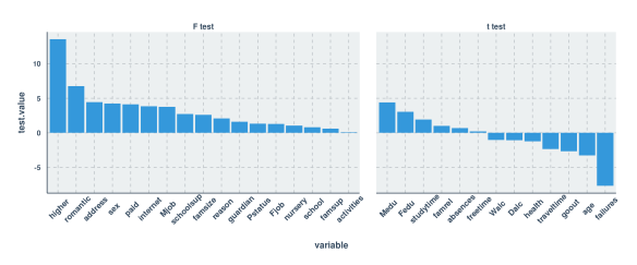
As you can see, the estimates that I generated in both languages were thankfully the same. My next thought was to use only those variables with a test value (F or t) of 3.0 or higher. What you’ll see below is that this led to a pretty severe decrease in predictive power compared to being liberal with feature selection.

In reality, the feature selection I use below shouldn’t be necessary at all given the size of the data set vs the number of predictors, and the statistical method that I’m using to predict grades (random forest). What’s more is that my feature selection method in fact led me to reject certain variables which I later found to be important in my expanded models! For this reason it would be nice to investigate a scalable multivariate feature selection method (I’ve been reading a bit about boruta but am skeptical about how well it scales up) to have in my tool belt. Enough blathering, and on with the model training:

Training the First Random Forest Model

#Python code
usevars =  [x for x in test_stats.query("test_value >= 3.0 | test_value <= -3.0")['variable']]
mat_perf['randu'] = np.array([uniform(0,1) for x in range(0,mat_perf.shape[0])])

mp_X = mat_perf[usevars]
mp_X_train = mp_X[mat_perf['randu'] <= .67]
mp_X_test = mp_X[mat_perf['randu'] > .67]

mp_Y_train = mat_perf.G3[mat_perf['randu'] <= .67]
mp_Y_test = mat_perf.G3[mat_perf['randu'] > .67]

# for the training set
cat_cols = [x for x in mp_X_train.columns if mp_X_train[x].dtype == "O"]
for col in cat_cols:
    new_cols = get_dummies(mp_X_train[col])
    new_cols.columns = col + '_' + new_cols.columns
    mp_X_train = concat([mp_X_train, new_cols], axis=1)

# for the testing set
cat_cols = [x for x in mp_X_test.columns if mp_X_test[x].dtype == "O"]
for col in cat_cols:
    new_cols = get_dummies(mp_X_test[col])
    new_cols.columns = col + '_' + new_cols.columns
    mp_X_test = concat([mp_X_test, new_cols], axis=1)

mp_X_train.drop(cat_cols, inplace=True, axis=1)
mp_X_test.drop(cat_cols, inplace=True, axis=1)

rf = RandomForestRegressor(bootstrap=True,
           criterion='mse', max_depth=2, max_features='auto',
           min_density=None, min_samples_leaf=1, min_samples_split=2,
           n_estimators=100, n_jobs=1, oob_score=True, random_state=None,
           verbose=0)
rf.fit(mp_X_train, mp_Y_train)

After I got past the part where I constructed the training and testing sets (with “unimportant” variables filtered out) I ran into a real annoyance. I learned that categorical variables need to be converted to dummy variables before you do the modeling (where each level of the categorical variable gets its own variable containing 1s and 0s. 1 means that the level was present in that row and 0 means that the level was not present in that row; so called “one-hot encoding”). I suppose you could argue that this puts less computational demand on the modeling procedures, but when you’re dealing with tree based ensembles I think this is a drawback. Let’s say you have a categorical variable with 5 features, “a” through “e”. It just so happens that when you compare a split on that categorical variable where “abc” is on one side and “de” is on the other side, there is a very significant difference in the dependent variable. How is one-hot encoding going to capture that? And then, your dataset which had a certain number of columns now has 5 additional columns due to the encoding. “Blah” I say!

Anyway, as you can see above, I used the get_dummies function in order to do the one-hot encoding. Also, you’ll see that I’ve assigned two thirds of the data to the training set and one third to the testing set. Now let’s see the same steps in R:

#R Code
keep.vars = match(filter(test.stats.df, abs(test.value) >= 3)$variable, names(mat_perf))
ctrl = trainControl(method="repeatedcv", number=10, selectionFunction = "oneSE")
mat_perf$randu = runif(395)
test = mat_perf[mat_perf$randu > .67,]
trf = train(mat_perf[mat_perf$randu <= .67,keep.vars], mat_perf$G3[mat_perf$randu <= .67],
            method="rf", metric="RMSE", data=mat_perf,
            trControl=ctrl, importance=TRUE)

Wait a minute. Did I really just train a Random Forest model in R, do cross validation, and prepare a testing data set with 5 commands!?!? That was a lot easier than doing these preparations and not doing cross validation in Python! I did in fact try to figure out cross validation in sklearn, but then I was having problems accessing variable importances after. I do like the caret package :) Next, let’s see how each of the models did on their testing set:

Testing the First Random Forest Model

#Python Code
y_pred = rf.predict(mp_X_test)
sns.set_context(context='poster', font_scale=1)
first_test = DataFrame({"pred.G3.keepvars" : y_pred, "G3" : mp_Y_test})
sns.lmplot("G3", "pred.G3.keepvars", first_test, size=7, aspect=1.5)
print 'r squared value of', stats.pearsonr(mp_Y_test, y_pred)[0]**2
print 'RMSE of', sqrt(mean_squared_error(mp_Y_test, y_pred))

R^2 value of 0.104940038879
RMSE of 4.66552400292

Here, as in all cases when making a prediction using sklearn, I use the predict method to generate the predicted values from the model using the testing set and then plot the prediction (“pred.G3.keepvars”) vs the actual values (“G3″) using the lmplot function. I like the syntax that the lmplot function from the seaborn package uses as it is simple and familiar to me from the R world (where the arguments consist of “X variable, Y Variable, dataset name, other aesthetic arguments). As you can see from the graph above and from the R^2 value, this model kind of sucks. Another thing I like here is the quality of the graph that seaborn outputs. It’s nice! It looks pretty modern, the text is very readable, and nothing looks edgy or pixelated in the plot. Okay, now let’s look at the code and output in R, using the same predictors.

#R Code
test$pred.G3.keepvars = predict(trf, test, "raw")
cor.test(test$G3, test$pred.G3.keepvars)$estimate[[1]]^2
summary(lm(test$G3 ~ test$pred.G3.keepvars))$sigma
ggplot(test, aes(x=G3, y=pred.G3.keepvars)) + geom_point() + stat_smooth(method="lm") + scale_y_continuous(breaks=seq(0,20,4), limits=c(0,20))

R^2 value of 0.198648
RMSE of 4.148194

Well, it looks like this model sucks a bit less than the Python one. Quality-wise, the plot looks super nice (thanks again, ggplot2 and ggthemr!) although by default the alpha parameter is not set to account for overplotting. The docs page for ggplot2 suggests setting alpha=.05, but for this particular data set, setting it to .5 seems to be better.

Finally for this section, let’s look at the variable importances generated for each training model:

#Python Code
importances = DataFrame({'cols':mp_X_train.columns, 'imps':rf.feature_importances_})
print importances.sort(['imps'], ascending=False)

             cols      imps
3        failures  0.641898
0            Medu  0.064586
10          sex_F  0.043548
19  Mjob_services  0.038347
11          sex_M  0.036798
16   Mjob_at_home  0.036609
2             age  0.032722
1            Fedu  0.029266
15   internet_yes  0.016545
6     romantic_no  0.013024
7    romantic_yes  0.011134
5      higher_yes  0.010598
14    internet_no  0.007603
4       higher_no  0.007431
12        paid_no  0.002508
20   Mjob_teacher  0.002476
13       paid_yes  0.002006
18     Mjob_other  0.001654
17    Mjob_health  0.000515
8       address_R  0.000403
9       address_U  0.000330

#R Code
varImp(trf)

## rf variable importance
## 
##          Overall
## failures 100.000
## romantic  49.247
## higher    27.066
## age       17.799
## Medu      14.941
## internet  12.655
## sex        8.012
## Fedu       7.536
## Mjob       5.883
## paid       1.563
## address    0.000

My first observation is that it was obviously easier for me to get the variable importances in R than it was in Python. Next, you’ll certainly see the symptom of the dummy coding I had to do for the categorical variables. That’s no fun, but we’ll survive through this example analysis, right? Now let’s look which variables made it to the top:

Whereas failures, mother’s education level, sex and mother’s job made it to the top of the list for the Python model, the top 4 were different apart from failures in the R model.

With the understanding that the variable selection method that I used was inappropriate, let’s move on to training a Random Forest model using all predictors except the prior 2 test scores. Since I’ve already commented above on my thoughts about the various steps in the process, I’ll comment only on the differences in results in the remaining sections.

Training and Testing the Second Random Forest Model

#Python Code

#aav = almost all variables
mp_X_aav = mat_perf[mat_perf.columns[0:30]]
mp_X_train_aav = mp_X_aav[mat_perf['randu'] <= .67]
mp_X_test_aav = mp_X_aav[mat_perf['randu'] > .67]

# for the training set
cat_cols = [x for x in mp_X_train_aav.columns if mp_X_train_aav[x].dtype == "O"]
for col in cat_cols:
    new_cols = get_dummies(mp_X_train_aav[col])
    new_cols.columns = col + '_' + new_cols.columns
    mp_X_train_aav = concat([mp_X_train_aav, new_cols], axis=1)
    
# for the testing set
cat_cols = [x for x in mp_X_test_aav.columns if mp_X_test_aav[x].dtype == "O"]
for col in cat_cols:
    new_cols = get_dummies(mp_X_test_aav[col])
    new_cols.columns = col + '_' + new_cols.columns
    mp_X_test_aav = concat([mp_X_test_aav, new_cols], axis=1)

mp_X_train_aav.drop(cat_cols, inplace=True, axis=1)
mp_X_test_aav.drop(cat_cols, inplace=True, axis=1)

rf_aav = RandomForestRegressor(bootstrap=True, 
           criterion='mse', max_depth=2, max_features='auto',
           min_density=None, min_samples_leaf=1, min_samples_split=2,
           n_estimators=100, n_jobs=1, oob_score=True, random_state=None,
           verbose=0)
rf_aav.fit(mp_X_train_aav, mp_Y_train)

y_pred_aav = rf_aav.predict(mp_X_test_aav)
second_test = DataFrame({"pred.G3.almostallvars" : y_pred_aav, "G3" : mp_Y_test})
sns.lmplot("G3", "pred.G3.almostallvars", second_test, size=7, aspect=1.5)
print 'r squared value of', stats.pearsonr(mp_Y_test, y_pred_aav)[0]**2
print 'RMSE of', sqrt(mean_squared_error(mp_Y_test, y_pred_aav))

R^2 value of 0.226587731888
RMSE of 4.3338674965

Compared to the first Python model, the R^2 on this one is more than doubly higher (the first R^2 was .10494) and the RMSE is 7.1% lower (the first was 4.6666254). The predicted vs actual plot confirms that the predictions still don’t look fantastic compared to the actuals, which is probably the main reason why the RMSE hasn’t decreased by so much. Now to the R code using the same predictors:

#R code
trf2 = train(mat_perf[mat_perf$randu <= .67,1:30], mat_perf$G3[mat_perf$randu <= .67],
            method="rf", metric="RMSE", data=mat_perf,
            trControl=ctrl, importance=TRUE)
test$pred.g3.almostallvars = predict(trf2, test, "raw")
cor.test(test$G3, test$pred.g3.almostallvars)$estimate[[1]]^2
summary(lm(test$G3 ~ test$pred.g3.almostallvars))$sigma
ggplot(test, aes(x=G3, y=pred.g3.almostallvars)) + geom_point() + 
  stat_smooth() + scale_y_continuous(breaks=seq(0,20,4), limits=c(0,20))

R^2 value of 0.3262093
RMSE of 3.8037318

Compared to the first R model, the R^2 on this one is approximately 1.64 times higher (the first R^2 was .19865) and the RMSE is 8.3% lower (the first was 4.148194). Although this particular model is indeed doing better at predicting values in the test set than the one built in Python using the same variables, I would still hesitate to assume that the process is inherently better for this data set. Due to the randomness inherent in Random Forests, one run of the training could be lucky enough to give results like the above, whereas other times the results might even be slightly worse than what I managed to get in Python. I confirmed this, and in fact most additional runs of this model in R seemed to result in an R^2 of around .20 and an RMSE of around 4.2.

Again, let’s look at the variable importances generated for each training model:

#Python Code
importances_aav = DataFrame({'cols':mp_X_train_aav.columns, 'imps':rf_aav.feature_importances_})
print importances_aav.sort(['imps'], ascending=False)

                 cols      imps
5            failures  0.629985
12           absences  0.057430
1                Medu  0.037081
41      schoolsup_yes  0.036830
0                 age  0.029672
23       Mjob_at_home  0.029642
16              sex_M  0.026949
15              sex_F  0.026052
40       schoolsup_no  0.019097
26      Mjob_services  0.016354
55       romantic_yes  0.014043
51         higher_yes  0.012367
2                Fedu  0.011016
39     guardian_other  0.010715
37    guardian_father  0.006785
8               goout  0.006040
11             health  0.005051
54        romantic_no  0.004113
7            freetime  0.003702
3          traveltime  0.003341

#R Code
varImp(trf2)

## rf variable importance
## 
##   only 20 most important variables shown (out of 30)
## 
##            Overall
## absences    100.00
## failures     70.49
## schoolsup    47.01
## romantic     32.20
## Pstatus      27.39
## goout        26.32
## higher       25.76
## reason       24.02
## guardian     22.32
## address      21.88
## Fedu         20.38
## school       20.07
## traveltime   20.02
## studytime    18.73
## health       18.21
## Mjob         17.29
## paid         15.67
## Dalc         14.93
## activities   13.67
## freetime     12.11

Now in both cases we’re seeing that absences and failures are considered as the top 2 most important variables for predicting final math exam grade. It makes sense to me, but frankly is a little sad that the two most important variables are so negative :( On to to the third Random Forest model, containing everything from the second with the addition of the students’ marks on their second math exam!

Training and Testing the Third Random Forest Model

#Python Code

#allv = all variables (except G1)
allvars = range(0,30)
allvars.append(31)
mp_X_allv = mat_perf[mat_perf.columns[allvars]]
mp_X_train_allv = mp_X_allv[mat_perf['randu'] <= .67]
mp_X_test_allv = mp_X_allv[mat_perf['randu'] > .67]

# for the training set
cat_cols = [x for x in mp_X_train_allv.columns if mp_X_train_allv[x].dtype == "O"]
for col in cat_cols:
    new_cols = get_dummies(mp_X_train_allv[col])
    new_cols.columns = col + '_' + new_cols.columns
    mp_X_train_allv = concat([mp_X_train_allv, new_cols], axis=1)
    
# for the testing set
cat_cols = [x for x in mp_X_test_allv.columns if mp_X_test_allv[x].dtype == "O"]
for col in cat_cols:
    new_cols = get_dummies(mp_X_test_allv[col])
    new_cols.columns = col + '_' + new_cols.columns
    mp_X_test_allv = concat([mp_X_test_allv, new_cols], axis=1)

mp_X_train_allv.drop(cat_cols, inplace=True, axis=1)
mp_X_test_allv.drop(cat_cols, inplace=True, axis=1)

rf_allv = RandomForestRegressor(bootstrap=True, 
           criterion='mse', max_depth=2, max_features='auto',
           min_density=None, min_samples_leaf=1, min_samples_split=2,
           n_estimators=100, n_jobs=1, oob_score=True, random_state=None,
           verbose=0)
rf_allv.fit(mp_X_train_allv, mp_Y_train)

y_pred_allv = rf_allv.predict(mp_X_test_allv)
third_test = DataFrame({"pred.G3.plusG2" : y_pred_allv, "G3" : mp_Y_test})
sns.lmplot("G3", "pred.G3.plusG2", third_test, size=7, aspect=1.5)
print 'r squared value of', stats.pearsonr(mp_Y_test, y_pred_allv)[0]**2
print 'RMSE of', sqrt(mean_squared_error(mp_Y_test, y_pred_allv))

R^2 value of 0.836089929903
RMSE of 2.11895794845

Obviously we have added a highly predictive piece of information here by adding the grades from their second math exam (variable name was “G2″). I was reluctant to add this variable at first because when you predict test marks with previous test marks then it prevents the model from being useful much earlier on in the year when these tests have not been administered. However, I did want to see what the model would look like when I included it anyway! Now let’s see how predictive these variables were when I put them into a model in R:

#R Code
trf3 = train(mat_perf[mat_perf$randu <= .67,c(1:30,32)], mat_perf$G3[mat_perf$randu <= .67], 
             method="rf", metric="RMSE", data=mat_perf, 
             trControl=ctrl, importance=TRUE)
test$pred.g3.plusG2 = predict(trf3, test, "raw")
cor.test(test$G3, test$pred.g3.plusG2)$estimate[[1]]^2
summary(lm(test$G3 ~ test$pred.g3.plusG2))$sigma
ggplot(test, aes(x=G3, y=pred.g3.plusG2)) + geom_point() + 
  stat_smooth(method="lm") + scale_y_continuous(breaks=seq(0,20,4), limits=c(0,20))

R^2 value of 0.9170506
RMSE of 1.3346087

Well, it appears that yet again we have a case where the R model has fared better than the Python model. I find it notable that when you look at the scatterplot for the Python model you can see what look like steps in the points as you scan your eyes from the bottom-left part of the trend line to the top-right part. It appears that the Random Forest model in R has benefitted from the tuning process and as a result the distribution of the residuals are more homoscedastic and also obviously closer to the regression line than the Python model. I still wonder how much more similar these results would be if I had carried out the Python analysis by tuning while cross validating like I did in R!

For the last time, let’s look at the variable importances generated for each training model:

#Python Code
importances_allv = DataFrame({'cols':mp_X_train_allv.columns, 'imps':rf_allv.feature_importances_})
print importances_allv.sort(['imps'], ascending=False)

                 cols      imps
13                 G2  0.924166
12           absences  0.075834
14          school_GP  0.000000
25        Mjob_health  0.000000
24       Mjob_at_home  0.000000
23          Pstatus_T  0.000000
22          Pstatus_A  0.000000
21        famsize_LE3  0.000000
20        famsize_GT3  0.000000
19          address_U  0.000000
18          address_R  0.000000
17              sex_M  0.000000
16              sex_F  0.000000
15          school_MS  0.000000
56       romantic_yes  0.000000
27      Mjob_services  0.000000
11             health  0.000000
10               Walc  0.000000
9                Dalc  0.000000
8               goout  0.000000

#R Code
varImp(trf3)

## rf variable importance
## 
##   only 20 most important variables shown (out of 31)
## 
##            Overall
## G2         100.000
## absences    33.092
## failures     9.702
## age          8.467
## paid         7.591
## schoolsup    7.385
## Pstatus      6.604
## studytime    5.963
## famrel       5.719
## reason       5.630
## guardian     5.278
## Mjob         5.163
## school       4.905
## activities   4.532
## romantic     4.336
## famsup       4.335
## traveltime   4.173
## Medu         3.540
## Walc         3.278
## higher       3.246

Now this is VERY telling, and gives me insight as to why the scatterplot from the Python model had that staircase quality to it. The R model is taking into account way more variables than the Python model. G2 obviously takes the cake in both models, but I suppose it overshadowed everything else by so much in the Python model, that for some reason it just didn’t find any use for any other variable than absences.

Conclusion

This was fun! For all the work I did in Python, I used IPython Notebook. Being an avid RStudio user, I’m not used to web-browser based interactive coding like what IPython Notebook provides. I discovered that I enjoy it and found it useful for laying out the information that I was using to write this blog post (I also laid out the R part of this analysis in RMarkdown for that same reason). What I did not like about IPython Notebook is that when you close it/shut it down/then later reinitialize it, all of the objects that form your data and analysis are gone and all you have left are the results. You must then re-run all of your code so that your objects are resident in memory again. It would be nice to have some kind of convenience function to save everything to disk so that you can reload at a later time.

I found myself stumbling a lot trying to figure out which Python packages to use for each particular purpose and I tended to get easily frustrated. I had to keep reminding myself that it’s a learning curve to a similar extent as it was for me while I was learning R. This frustration should not be a deterrent from picking it up and learning how to do machine learning in Python. Another part of my frustration was not being able to get variable importances from my Random Forest models in Python when I was building them using cross validation and grid searches. If you have a link to share with me that shows an example of this, I’d be happy to read it.

I liked seaborn and I think if I spend more time with it then perhaps it could serve as a decent alternative to graphing in ggplot2. That being said, I’ve spent so much time using ggplot2 that sometimes I wonder if there is anything out there that rivals its flexibility and elegance!

The issue I mentioned above with categorical variables is annoying and it really makes me wonder if using a Tree based R model would intrinsically be superior due to its automatic handling of categorical variables compared with Python, where you need to one-hot encode these variables.

All in all, I hope this was as useful and educational for you as it was for me. It’s important to step outside of your comfort zone every once in a while :)

Last Friday at the Davis R Users’ Group, Mallory Johnson gave a presentation on RQDA, an R-based GUI tool for doing coding on documents for use in qualitative text analysis. Here’s the video, and you can view the slides here

[Sorry about reverb in the video]

Resources

• The RQDA home page
• More RQDA instructional videos

ANXA11 expression in human smooth muscle aortic cells post-ILb1 exposure

I was very impressed by maSigPro and meant to get around to writing a short guide showing how to use it. So I did finally, using RMarkdown to create the document and here it is. The document also illustrates how to retrieve datasets from GEO using GEOquery and annotate microarray probesets using biomaRt. Hopefully it’s useful to some of you.

I’ll probably do more of this in the future, since publishing RMarkdown to RPubs is far easier than copying, pasting and formatting at WordPress.

library(packcircles)
library(ggplot2)
library(gridExtra)

# Generate some random overlapping circles
ncircles <- 200
limits <- c(-50, 50)
inset <- diff(limits) / 3
rmax <- 20

xyr <- data.frame(
  x = runif(ncircles, min(limits) + inset, max(limits) - inset),
  y = runif(ncircles, min(limits) + inset, max(limits) - inset),
  r = rbeta(ncircles, 1, 10) * rmax)

# Index of the largest circle
largest.id <- which(xyr$r == max(xyr$r))

## Generate plot data for the `before` layout
dat.before <- circlePlotData(xyr)

# Add a column to the plot data for the 'before' circles
# to indicate whether a circle is static of free to move
dat.before$state <- ifelse(dat.before$id == largest.id, "static", "free")

# Run the layout algorithm with a weights vector to fix the position
# of the largest circle
wts <- rep(1.0, nrow(xyr))
wts[ largest.id ] <- 0.0

res <- circleLayout(xyr, limits, limits, maxiter = 1000, weights=wts)

# A plot function to colour circles based on the state column
doPlot <- function(dat, title)
  ggplot(dat) + 
  geom_polygon(aes(x, y, group=id, fill=state), colour="brown1") +
  scale_fill_manual(values=c("NA", "brown4")) +
  coord_equal(xlim=limits, ylim=limits) +
  theme_bw() +
  theme(axis.text=element_blank(),
        axis.ticks=element_blank(),
        axis.title=element_blank(),
        legend.position="none") +
  labs(title=title)

g.before <- doPlot(dat.before, "before")

# Generate a plot for the 'after' circles
dat.after <- circlePlotData(res$layout)
dat.after$state <- ifelse(dat.after$id == largest.id, "static", "free")

g.after <- doPlot(dat.after, "after")

grid.arrange(g.before, g.after, nrow=1)

I’m in Rome at the International Workshop on Computational Economics and Econometrics. I gave a seminar on Monday on the ever-popular subject of data visualization. Slides are here. In a few minutes, I’ll be speaking on Inference in Complex Systems, a topic of some interest from practical research experience my colleague Rick Hood and I have had in health and social care research.

Here’s a link to my handout for that: iwcee-handout

In essence, we draw on realist evaluation and mixed-methods research to emphasise understanding the complex system and how the intervention works inside it. Unsurprisingly for regular readers, I try to promote transparency around subjectivities, awareness of philosophy of science, and Bayesian methods.

This Tuesday, I will be in Leuven (in Belgium) at the ACP meeting to give  a talk on Data Science: from Small to Big Data. The talk will take place in the Faculty Club from 6 till 8 pm. Slides could be found online (with animated pictures).

As usual, comments are welcome.

testthat 0.10.0 is now available on CRAN. Testthat makes it easy to turn the informal testing that you’re already doing into formal automated tests. Learn more at http://r-pkgs.had.co.nz/tests.html. Install the latest version with:

install.packages("testthat")

There are four big changes in this release:

• test_check() uses a new reporter specifically designed for R CMD check. It displays a summary at the end of the tests, designed to be <13 lines long so test failures in R CMD check display are as useful as possible.
• New skip_if_not_installed() skips tests if a package isn’t installed: this is useful if you want tests to skip if a suggested package isn’t installed.
• The expect_that(a, equals(b)) style of testing has been soft-deprecated in favour of expect_equals(a, b). It will keep working, but it’s no longer demonstrated in the documentation, and new expectations will only be available in expect_equal(a, b) style.
• compare() is now documented and exported: compare is used to display test failures for expect_equal(), and is designed to help you spot exactly where the failure occured. It currently has methods for character and numeric vectors.

There were a number of other minor improvements and bug fixes. See the release notes for a complete list.

29.05.2015

I published a MacOSX release candidate for Bio7 2.1 based on Eclipse 4.5 RC2. This release was tested on MacOSX 10.10. The final release will be published after the official Eclipse 4.5 release.

Installation:

• Bio7 2.1 comes as a regular *.dmg installation package. Just drag the Bio7.app to the Applications folder.
• Bio7 2.1 comes with a bundled jre 1.8.45. No need to install an extra Java Runtime Environment.
• Bio7 2.1 comes bundled with R 3.2.0 and Rserve 1.8.2 installed.

Eventually XQuartz has to be installed to use the default custom R plotting device of Bio7 on MacOSX. If you plot the first time with R and XQuartz is not available a dialog will inform about the missing package.

Download Bio7 at:

http://bio7.org

By Andy Nicholls, Head of Consulting

As companies increasingly look beyond the scope of what is logistically possible in Excel more and more companies are approaching Mango looking for help with connecting to Excel from R. With over 6,500 packages now on CRAN it should come as no surprise that there are quite a few packages that have be written in order to connect to Excel from R. So which is the best? Unfortunately it really does depend on what you want to do but here’s a quick guide to some of the main packages available from CRAN.

The “All-Rounders”

Overview

There are four “all-rounder” packages that can both read and write to Excel: XLConnect written and maintained by Mirai Solutions; xlsx by Adrian Dragulescu; openxlsx by Alexander Walker; excel.link by Gregory Demin. With each of these packages it is possible to follow a structured workflow in which a user connects to a workbook, extracts data, processes the data in R and then writes back data, graphics or even Excel formulae back to the workbook. It is possible to add new sheets, recolour, add formulae and so on. There are however some important differences that users should be aware of.

Formal Comparison of “All-Rounders”

At Mango we regularly run tests to assess developments around these packages in order to assess their suitability for various projects. The test is fairly straightforward and simply involves connecting to a 4MB file, reading in some different data formats and writing back data and graphics to the spreadsheet.  The results are shown in the table below.

General Observations

For the general consumer I personally think XLConnect is the best all-rounder though functionally there’s not much difference between this and xlsx. Both XLConnect and xlsx depend on rJava but the Java elements are hidden away from the user with XLConnect and primarily for that reason I have a slight personal preference for XLConnect. If your workbook is full of “=sum()” or other formulae then it is also worth noting that XLConnect will read in the result of the calculation whereas xlsx interprets the formula as NA. Personally I am not a big fan of the XLConnect header formatting when writing data to Excel however. If you’re an xlsx pro user though there’s certainly no reason that I can think of to drop the package and switch to XLConnect.

One potential downside of both XLConnect and xlsx is their Java dependency. Users with medium to large workbooks may soon encounter “Java heap space” error messages as memory is consumed in huge quantities. Those working for companies where IT have ultimate rule over your laptop may also find it difficult to get set up in the first place by ensuring that Java is installed and available in the right location. This is essentially a binary hurdle that you can either overcome or you can’t. If you can it’s worth continuing as these are geat packages.

openxlsx is fairly new and a package that I hadn’t tried until recently. I have to say I’ve been impressed with what I’ve seen thus far. Crucially it does not have a dependency on Java though Windows users will need a zip application (eg Rtools). The functionality and consistency is not quite at the level of XLConnect or xlsx yet. For example the read.xlsx has startRow argument but no startCol. You can use the argument cols to specify start and end columns but it feels more like a workaround in my opinion. Dates are read in as numeric by default as well which most users will find frustrating (unlike XLConnect or xlsx which convert dates to POSIXct). Plus it’s noticabley slower than the aforementioned packages for large workbooks. Despite all of that however, it is the only all-rounder package that I’ve used that can easily connect to and import a protected sheet from a large “xlsm” test file that we have at Mango, pumped full of VBA. And for what it’s worth it is also the only all-rounder that interprets a “#NUM” in Excel as NaN in R; XLConnect and xlsx read such values as NA whilst excel.link fails with an error. Graphics may also be written directly to Excel without having to generate an intermediate file (though often an intermediate file can be a useful output).

That leaves excel.link. I left this one until last as it’s very different from the other three all-rounder packages. excel.link uses RDCOMClient and any edits to a workbook are live edits in an open workbook, making it easier to develop a script. It also passes Mango’s “xlsm” test, albeit only after the protected sheet is unprotected. However it’s quite tough to pick up for the lay-user and for some reason it doesn’t appear to be able to read hidden sheets. Speed is also an issue that users will notice if their script is particularly long and the workbook large. That said it certainly offers something different to the other packages however and if you learn it well then it’s a powerful ally.

Reading Structured Data from Excel

The all-rounders are great but if you are fortunate enough to have structured data, which in this context means your datasets are stored in the top left-hand corner of separate tabs, then there are a few other options to consider which may be much faster than the ‘all-rounder’ packages for reading in data. The multi-purpose RODBC is very mature and really easy to use but some users can be limited by their driver set-up. RJDBC is a viable, albeit slower alternative that has it’s own (Java) restriction. Hadley Wickham has a habit of finding problems that need solving and for those who are struggling with either of these packages readxl is the new kid on the block for structured data that everyone will probably be using by the end of the year.

What Else is There?

There are further specific packages available such as Guido van Steen’s dataframes2xls package which uses Python’s pyexcelerator to write to xls and Marc Schartz’s WriteXLS which uses Perl to write to xls and xlsx files. Another Perl implemntation is Gregory Warnes’s gdata which can be used to read data from Excel. And the list goes on but I have to stop writing at some point!

Conclusion

If you’ve found a good package stick to it! If you’re starting out it’s worth considering the structure of your data and the end users of your code. Are they going to have all the freedom you have to configure Java, install drivers and so on?  There are plenty of packages available and most of them are pretty good so long as you understand their limitations.

INCOME PERCENTILES AND INCOMES PAINT DIFFERENT PICTURES

The amazing team at the New York Times have a “You Draw It” feature in The Upshot in which readers try their hands at drawing a graph. The graph should show the probability of a child going to college based on their parents’ percentile in the income distribution.

As a cool added feature, after people took their guesses, they could see, in shades of red, the other guesses people had taken and compare it to the actual graph.

SPOILER ALERT: You can see the true answer at the bottom of this post. If you want to try your hand at guessing, click through to the NY Times and guess before proceeding.

One way to interpret this relationship is that for every percentile a parent moves up in the income distribution, the chance that their child goes to college increases by a constant amount, which might seem somewhat surprising. Even the NY Times editors were surprised by this linear relationship, and the data they collected showed that other people were, too.

Jake Hofman and I wondered “what if people didn’t take the X-axis literally, what if they thought about it as something like log income or income (instead of percentile in the income distribution)?” Percentiles are tricky. They’re buckets with equal numbers of people, but those people can have very different incomes. What would the graph look like if the X-axis were income? Would this relationship be more intuitive to readers?

Jake scraped some income percentile data from whatsmypercent.com and we eyeballed the probability data from the chart at the NY Times. This enabled us to look at the probability of going to college based on income, which tells somewhat of a different story. In these plots, the size of the each point corresponds to the number of people in it.

The change you get by adding $10,000 a family’s income matters considerably for those earning between $10,000 and $100,000 (which the vast majority of Americans do), and matters much less outside that range. At the same time, it’s considerably more difficult for lower income parents to increase their income by this amount.

Probability of going to college vs log income:

Probability of going to college vs income:

SPOILER ALERT – BELOW YOU WILL SEE THE ANSWER FROM THE NY TIMES

Probability of going to college vs income percentile:

R CODE FOR YOUR CODING PLEASURE

The post Chances of going to college based on parent’s income appeared first on Decision Science News.

In blog posts a few months ago, I proposed an alternative to MapReduce, e.g. to Hadoop, which I called “Snowdoop.” I pointed out that systems like Hadoop and Spark are very difficult to install and configure, are either too primitive (Hadoop)  or too abstract (Spark) to program, and above all, are SLOW. Spark is of course a great improvement on Hadoop, but still suffers from these problems to various extents.

The idea of Snowdoop is to

• retain the idea of Hadoop/Spark to work on top of distributed file systems (“move the computation to the data rather than vice versa”)
• work purely in R, using familiar constructs
• avoid using Java or any other external language for infrastructure
• sort data only if the application requires it

I originally proposed Snowdoop just as a concept, saying that I would slowly develop it into an actual package. I later put the beginnings of a Snowdoop package in a broader package, partools, which also contains other parallel computation utilities, such as a debugging aid for the cluster portion of R’s parallel package (which I like to call Snow, as it came from the old snow package).

I remain convinced that Snowdoop is a much more appropriate tool for many R users who are currently using Hadoop or Spark. The latter two, especially Spark, may be a much superior approach for those with very large clusters, thus with a need for built-in fault tolerance (Snowdoop provides none on its own), but even the Hadoop Wiki indicates that many MapReduce users actually work on clusters of very modest size.

So, in the last few weeks, I’ve added quite a bit to Snowdoop, and have run more timing tests. The latter are still very preliminary, but they continue to be very promising. In this blog post, I’ll give an extended example of usage of the latest version, which you can obtain from GitHub. (I do have partools on CRAN as well, but have not updated that yet.)

The data set in this example will be the household power usage data set from UCI. Most people would not consider this “Big Data,” with only about 2 million rows and 9 columns, but it’s certainly no toy data set, and it will make serve well for illustration purposes.

But first, an overview of partools:

• distributed approach, either persistent (distributed files) or quasi-persistent (distributed objects at the cluster nodes, in memory but re-accessed repeatedly)
• most Snowdoop-specific function names have the form file*
• most in-memory functions have names distrib*
• misc. functions, e.g. debugging aid and “Software Alchemy”

Note that partools, therefore, is more than just Snowdoop.  One need not use distributed files, and simply use the distrib* functions as handy ways to simplify one’s parallel code.

So, here is a session with the household power data.  I’m running on a 16-core machine, using 8 of the cores. For convenience, I changed the file name to hpc.txt. We first create the cluster, and initialize partools, e.g. assign an ID number to each cluster node:

 
> cls <- makeCluster(8)
> setclsinfo(cls) # partools call

Next we split the file into chunks, using the partools function filesplit() (done only once, not shown here). This creates files hpc.txt.1, hpc.txt.2 and so on (in this case, all on the same disk). Now have each cluster node read in its chunk:

> system.time(clusterEvalQ(cls,hp <-    read.table(filechunkname("hpc.txt",1),
header=TRUE,sep=";",stringsAsFactors=FALSE)))
 user system elapsed
 9.468 0.270 13.815

(Make note of that time.) The partools function filechunkname() finds the proper file chunk name for the calling cluster node, based on the latter’s ID. We now have a distributed data frame, named hp at each cluster node.

The package includes a function distribagg(), a distributed analog of R’s aggregate() function.  Here is an example of use, first converting the character variables to numeric:

> clusterEvalQ(cls,for (i in 3:9) hp[,i] <- as.numeric(hp[,i]))
> system.time(hpoutdis <-distribagg(cls,"x=hp[,3:6],
   by=list(hp[,7],hp[,8])","max",2))
 user system elapsed
 0.194 0.017 9.918

As you can see, the second and third arguments to distribagg() are those of aggregate(), in string form.

Now let’s compare to the serial version:

> system.time(hp <- read.table("hpc.txt",header=TRUE,sep=";",
stringsAsFactors=FALSE))
 user system elapsed
 22.343 0.175 22.529
> for (i in 3:9) hp[,i] <- as.numeric(hp[,i])
> system.time(hpout <- aggregate(x=hp[,3:6],by=list(hp[,7],hp[,8]),FUN=max))
 user system elapsed
 76.348 0.184 76.552

So, the computation using distribagg() was almost 6 times faster than serial, a good speed for 8 cluster nodes. Even the input from disk was more than twice as fast, in spite of the files being on the same disk, going through the same operating system.

This chapter is on what I call fold-vectorization. In some languages, it’s called reduce, though the concept is the same. Fold implements binary iterated function application, where elements of a sequence are passed along with an accumulator to a function. This process repeats such that each successive element is paired with the previous result of the function application. The version of fold discussed in the book appears in my lambda.tools package.

There are numerous applications of fold that span basic algebraic functions, such as the cumulative sum and product, to applying the derivative, to implementing Markov Chains. This chapter first delves into the mathematical motivation for fold. It then returns to the ebola.sitrep package and discusses the use of fold for applying transformations to data frames. Some examples work off the parsed file, which resides in the data directory of the project. The chapter finishes up by reviewing some methods of numerical analysis related to function approximation and series to further illustrate the use of fold in implementing mathematical relationships.

As usual, feedback and comments are welcome. I’m mostly interested in conceptual issues, although grammatical and typographical issues are also fair game.

Rowe – Modeling Data With Functional Programming Chs1-4

I first became interested in networks when reading Matthew O’Jackson’s 2010 paper describing networks in economics. At some point during the 2014 ebola outbreak, I became interested in how the disease could actually come to the U.S. I was caught up with work/classes at the time, but decided to use airline flight data to at least explore the question.

This is the same dataset I used here. The datasource is given in that post.

I assumed that the disease had a single origin (Liberia) and wanted to explore the question of how fast the disease could travel to the U.S.

A visualization of the network can be seen below. Each node is a country and each edge represents an existing airline route from one country to another. Flights that take off and land in the same country are omitted to avoid clutter.

Communities and Homophily

I used a spinglass algorithm to detect “communities” of countries, i.e. sets of countries with many flights between themselves, but few flights between them and countries not in the set. Roughly speaking, the algorithm tended to group countries in the same continent together. However, this is not always the case. For example, France was was placed in the same community as several African countries, due to the close relationships with its former colonies. Roughly speaking, this network seems to exhibit homophily – where countries on the same continent tend to be connected more with each other than with countries off their continent.

Liberia, the US, and Degree Distribution

The labels are unclear in the plot, but the United States and Liberia are in two separate communities, which may lead us to believe that Ebola spreading from the former to the latter would be unlikely. In fact, the degrees (number of countries a given country is connected to) of the countries differ greatly, which would also support this intuition. The US is connected to 186 other countries, whereas Liberia is connected to only 12. The full degree distribution is shown below. It roughly follows a power law, which, according to wikipedia, is what we should expect. Note that the approximation is asymptotic, which could be why this finite sample is off. According to the degree distribution, half of all countries are connected to 27 other countries. Liberia falls far below the median and the US falls far above the median.

Small Worlds

Let’s zoom in and look at Liberia’s second-degree connections:

Even though they’re in two different communities, Liberia and the US are only two degrees of separation away. This is generally case for all countries. If, for each node, we calculated the shortest path between it and every other node, the average shortest distance would be about 2 (specifically 2.3) hops. This is called the small world phenomenon. On average, every country is 2 hops away from every other country. Many networks exhibit this phenomenon largely due to “hubs” – countries (more generally, nodes) with lots of connections to other countries. For example, you can imagine that Charles de Gaulle airport in France is a hub, which links countries in the US, Eastern Europe, Asia, and Africa. The existence of these hubs makes it possible to get from one country to another with very few transfers.

Contagion

The close-up network above shows that if ebola were to spread to the US, it might be through Nigeria, Ghana, Morocco, and Belgium. If we knew the proportion of flights that went from liberia to each of these countries and from each of these countries to the US, we could estimate the probability of Ebola spreading for each route. I don’t have time to do this, although it’s certainly possible given the data.

Of course, this is a huge simplification for many reasons. Even though Sierra Leon, for example, doesn’t have a direct connection to the US, it could be connected to other countries that are connected to the US. This route could have a very high proportion of flights end up in the US. So we would need to account for this factor.

There are also several epidemiological parameters that could change how quickly the disease spreads. For example, the length of time from infection to symptoms is important. If the infected don’t show symptoms until a week after infection, then they can’t be screened and contained as easily. They could infect many others before showing symptoms.

The deadliness of the disease is also important. If patients die within hours of being infected, then the disease can’t spread very far. To take the extreme, consider a patient dies within a second of being infected. Then there’s very little time for him to infect others.

Finally, we assumed a single origin. If the disease is already present in several countries when we run this analysis, then we would have to factor in multiple origins.

routes=read.table('.../routes.dat',sep=',')
ports=read.table('.../airports.dat',sep=',')

library(igraph)

# for each flight, get the country of the airport the plane took off from and landed at.
ports=ports[,c('V4','V5')]
names(ports)=c('country','airport')

routes=routes[,c('V3','V5')]
names(routes)=c('from','to')

m=merge(routes,ports,all.x=TRUE,by.x=c('from'),by.y=c('airport'))
names(m)[3]=c('from_c')
m=merge(m,ports,all.x=TRUE,by.x=c('to'),by.y=c('airport'))
names(m)[4]=c('to_c')

m$count=1
# create a unique country to country from/to route ID
m$id=paste(m$from_c,m$to_c,sep=',')

# see which routes are flown most frequently
a=aggregate(m$count,list(m$id),sum)
names(a)=c('id','flights')
a$fr=substr(a$id,1,regexpr(',',a$id)-1)
a$to=substr(a$id,regexpr(',',a$id)+1,100)
a=a[,2:4]

a$perc=(a$flights/sum(a$flights))*100

# create directed network graph
a=a[!(a[,2]==a[,3]),]
mat=as.matrix(a[,2:3])

g=graph.data.frame(mat, directed = T)

edges=get.edgelist(g)
deg=degree(g,directed=TRUE)
vv=V(g)

# use spinglass algo to detect community
set.seed(9)
sgc = spinglass.community(g)
V(g)$membership=sgc$membership
table(V(g)$membership)

V(g)[membership==1]$color = 'pink'
V(g)[membership==2]$color = 'darkblue'
V(g)[membership==3]$color = 'darkred'
V(g)[membership==4]$color = 'purple'
V(g)[membership==5]$color = 'darkgreen'

plot(g,
     main='Airline Routes Connecting Countries',
     vertex.size=5,
     edge.arrow.size=.1,
     edge.arrow.width=.1,
     vertex.label=ifelse(V(g)$name %in% c('Liberia','United States'),V(g)$name,''),
     vertex.label.color='black')
legend('bottomright',fill=c('darkgreen','darkblue', 'darkred', 'pink', 'purple'),
       c('Africa', 'Europe', 'Asia/Middle East', 'Kiribati, Marshall Islands, Nauru', 'Americas'),
       bty='n')

# plot degree distribution
dplot=degree.distribution(g,cumulative = TRUE)

plot(dplot,type='l',xlab='Degree',ylab='Frequency',main='Degree Distribution of Airline Network',lty=1)
lines((1:length(dplot))^(-.7),type='l',lty=2)
legend('topright',lty=c(1,2),c('Degree Distribution','Power Law with x^(-.7)'),bty='n')

# explore membership...regional patterns exist
cc=cbind(V(g)$name,V(g)$membership)
tt=cc[cc[,2]==5,]

# explort connection from Liberia to United States
m=mat[mat[,1]=='Liberia',]

t=mat[mat[,1] %in% m[,2],]
tt=t[t[,2]=='United States',]

# assess probabilities

lib=a[a$fr=='Liberia',]
lib$prob=lib$flights/sum(lib$flights)
  # most probable route from liberia is Ghana

vec=c(tt[,1],'Liberia')
names(vec)=NULL

g2=graph.data.frame(mat[(mat[,1] %in% vec & mat[,2] == 'United States') | (mat[,1]=='Liberia'),], directed = T)
V(g2)$color=c('darkblue','darkgreen','darkgreen','darkgreen','darkgreen','purple','darkgreen','darkgreen')

plot(g2,
     main='Airline Connections from Liberia to the United States',
     vertex.size=5,
     edge.arrow.size=1,
     edge.arrow.width=.5,
     vertex.label.color='black')
legend('bottomright',fill=c('darkgreen','darkblue','purple'),
       c('Africa', 'Europe', 'Americas'),
       bty='n')


aa=a[a$fr %in% tt[,1],]
sum=aggregate(aa$flights,list(aa$fr),sum)

bb=a[a$fr %in% tt[,1] & a$to=='United States',]

fin=data.frame(bb$fr,sum$x,bb$flights,bb$flights/sum$x)

s=shortest.paths(g)
mean(s)

My wife got me a Safe Cracker 40 puzzle a while back. I believe I misplaced the solution some time back. The company, Creative Crafthouse, stands behind their products. They had amazing customer service and promptly supplied me with a solution. I’d supply the actual wheels as a cutout paper version but this is their property so this blog will be more enjoyable if you buy yourself a Safe Cracker 40 as well (I have no affiliation with the company, just enjoy their products and they have great customer service). Here’s what the puzzle looks like:

There are 26 columns of 4 rows. The goal is to line up the dials so you have all columns summing to 40. It is somewhat difficult to explain how the puzzle moves, but the dials control two rows. The outer row of the dial is notched and only covers every other cell of the row below. The outer most row does not have a notched row covering it. I believe there are 16^4 = 65536 possible combinations. I think it’s best to understand the logic by watching the video:

I enjoy puzzles but after a year didn’t solve it. This one begged me for a computer solution, and so I decided to use R to force the solution a bit. To me the computer challenge was pretty fun in itself.

Here are the dials. The NAs represents the notches in the notched dials. I used a list structure because it helped me sort things out. Anything in the same list moves together, though are not the same row. Row a is the outer most wheel. Both b and b_1 make up the next row, and so on.

L1 <- list(#outer
    a = c(2, 15, 23, 19, 3, 2, 3, 27, 20, 11, 27, 10, 19, 10, 13, 10),
    b = c(22, 9, 5, 10, 5, 1, 24, 2, 10, 9, 7, 3, 12, 24, 10, 9)
)
L2 <- list(
    b_i = c(16, NA, 17, NA, 2, NA, 2, NA, 10, NA, 15, NA, 6, NA, 9, NA),
    c = c(11, 27, 14, 5, 5, 7, 8, 24, 8, 3, 6, 15, 22, 6, 1, 1)
)
L3 <- list(
    c_j = c(10, NA, 2,  NA, 22, NA, 2,  NA, 17, NA, 15, NA, 14, NA, 5, NA),
    d = c( 1,  6,  10, 6,  10, 2,  6,  10, 4,  1,  5,  5,  4,  8,  6,  3) #inner wheel
)
L4 <- list(#inner wheel
    d_k = c(6, NA, 13, NA, 3, NA, 3, NA, 6, NA, 10, NA, 10, NA, 10, NA)
)

This is a brute force method but is still pretty quick. I made a shift function to treat vectors like circles or in this case dials. Here’s a demo of shift moving the vector one rotation to the right.

"A" "B" "C" "D" "E" "F" "G" "H" "I" "J"

results in:

"J" "A" "B" "C" "D" "E" "F" "G" "H" "I" 

I use some indexing of the NAs to over write the notched dials onto each of the top three rows.

shift <- function(x, n){
    if (n == 0) return(x)
    c(x[(n+1):length(x)], x[1:n])
}

dat <- NULL
m <- FALSE

for (i in 0:15){ 
    for (j in 0:15){
        for (k in 0:15){

            # Column 1
            c1 <- L1[[1]]  

            # Column 2
            c2 <- L1[[2]]  
            c2b <- shift(L2[[1]], i)
            c2[!is.na(c2b)]<- na.omit(c2b)

            # Column 3
            c3 <- shift(L2[[2]], i)
            c3b <- shift(L3[[1]], j)
            c3[!is.na(c3b)]<- na.omit(c3b)

            # Column 4
            c4 <- shift(L3[[2]], j)
            c4b <- shift(L4[[1]], k)
            c4[!is.na(c4b)]<- na.omit(c4b)

            ## Check and see if all rows add up to 40
            m <- all(rowSums(data.frame(c1, c2, c3, c4)) %in% 40)

            ## If all rows are 40 print the solution and assign to dat
            if (m){
                assign("dat", data.frame(c1, c2, c3, c4), envir=.GlobalEnv)
                print(data.frame(c1, c2, c3, c4))
                break
            }
            if (m) break
        }    
        if (m) break
    }
    if (m) break
}

Here’s the solution:

   c1 c2 c3 c4
1   2  6 22 10
2  15  9  6 10
3  23  9  2  6
4  19 10  1 10
5   3 16 17  4
6   2  1 27 10
7   3 17 15  5
8  27  2  5  6
9  20  2 14  4
10 11  9  7 13
11 27  2  5  6
12 10  3 24  3
13 19 10 10  1
14 10 24  3  3
15 13 15  2 10
16 10  9 15  6

We can check dat (I wrote the solution the global environment) with rowSums:

 rowSums(dat)
 [1] 40 40 40 40 40 40 40 40 40 40 40 40 40 40 40 40

A fun exercise for me. If anyone has a more efficient and/or less code intensive solution I’d love to hear about it.

Somehow almost an entire academic year went by without a blog post, I must have been busy… It’s time to get back in the saddle! (I’m using the classical definition of this idiom here, “doing something you stopped doing for a period of time”, not the urban dictionary definition, “when you are back to doing what you do best”, as I really don’t think writing blog posts are what I do best…)

One of the exciting things I took part in during the year was the NSF supported Reproducible Science Hackathon held at NESCent in Durham back in December.

I wrote here a while back about making reproducibility a central focus of students’ first introduction to data analysis, which is an ongoing effort in my intro stats course. The hackathon was a great opportunity to think about promoting reproducibility to a much wider audience than intro stat students — wider with respect to statistical background, computational skills, and discipline. The goal of the hackathon was to develop a two day workshop for reproducible research, or more specifically, reproducible data analysis and computation. Materials from the hackathon can be found here and are all CC0 licensed.

If this happened in December, why am I talking about this now? I was at USCOTS these last few days, and lead a breakout session with Nick Horton on reproducibility, building on some of the materials we developed at the hackathon and framing them for a stat ed audience. The main goals of the session were

1. to introduce statistics educators to RMarkdown via hands on exercises and promote it as a tool for reproducible data analysis and
2. to demonstrate that with the right exercises and right amount of scaffolding it is possible (and in fact easier!) to teach R through the use of RMarkdown, and hence train new researchers whose only data analysis workflow is a reproducible one.

In the talk I also discussed briefly further tips for documentation and organization as well as for getting started with version control tools like GitHub. Slides from my talk can be found here and all source code for the talk is here.

There was lots of discussion at USCOTS this year about incorporating more analysis of messy and complex data and more research into the undergraduate statistics curriculum. I hope that there will be an effort to not just do “more” with data in the classroom, but also do “better” with it, especially given that tools that easily lend themselves to best practices in reproducible data analysis (RMarkdown being one such example) are now more accessible than ever.

On this blog, I've had a long running investigation/demonstration of how to make a "embarrassingly-parallel" but computationally intractable (on commodity hardware, at least) R problem more performant by using parallel computation and Rcpp.

The example problem is to find the mean distance between every airport in the United States. This silly example was chosen because it exhibits polynomial growth in running time as a function of the number of airports and, thus, quickly becomes intractable without sampling. It is also easy to parallelize.

The first post used the (now-deprecated in favor of 'parallel') multicore package to achieve a substantial speedup. The second post used Rcpp to achieve a statistically significant but, functionally, trivial speedup by replacing the inner loop (the distance calculation using the Haversine formula) with a version written in C++ using Rcpp. Though I was disappointed in the results, it should be noted that porting the function to C++ took virtually no extra work.

By necessity, I've learned a lot more about high-performance R since writing those two posts (part of this is by trying to make my own R package as performant as possible). In particular, I did the Rcpp version all wrong, and I'd like to rectify that in this post. I also compare the running times of approaches that use both parallelism and Rcpp.

Lesson 1: use Rcpp correctly
The biggest lesson I learned, is that it isn’t sufficient to just replace inner loops with C++ code; the repeated transferring of data from R to C++ comes with a lot of overhead. By actually coding the loop in C++, the speedups to be had are often astounding.

In this example, the pure R version, that takes a matrix of longitude/latitude pairs and computed the mean distance between all combinations, looks like this...

just.R <- function(dframe){
  numrows <- nrow(dframe)
  combns <- combn(1:nrow(dframe), 2)
  numcombs <- ncol(combns)
  combns %>%
  {mapply(function(x,y){
          haversine(dframe[x,1], dframe[x,2],
                    dframe[y,1], dframe[y,2]) },
          .[1,], .[2,])} %>%
  sum %>%
  (function(x) x/(numrows*(numrows-1)/2))
}

The naive usage of Rcpp (and the one I used in the second blog post on this topic) simply replaces the call to "haversine" with a call to "haversine_cpp", which is written in C++. Again, a small speedup was obtained, but it was functionally trivial.

The better solution is to completely replace the combinations/"mapply" construct with a C++ version. Mine looks like this...

double all_cpp(Rcpp::NumericMatrix& mat){
    int nrow = mat.nrow();
    int numcomps = nrow*(nrow-1)/2;
    double running_sum = 0;
    for( int i = 0; i < nrow; i++ ){
        for( int j = i+1; j < nrow; j++){
            running_sum += haversine_cpp(mat(i,0), mat(i,1),
                                         mat(j,0), mat(j,1));
        }
    }
    return running_sum / numcomps;
}

The difference is incredible…

res <- benchmark(R.calling.cpp.naive(air.locs[,-1]),
                 just.R(air.locs[,-1]),
                 all_cpp(as.matrix(air.locs[,-1])),
                 columns = c("test", "replications", "elapsed", "relative"),
                                  order="relative", replications=10)
res
#                                   test replications elapsed relative
# 3  all_cpp(as.matrix(air.locs[, -1]))           10   0.021    1.000
# 1 R.calling.cpp.naive(air.locs[, -1])           10  14.419  686.619
# 2              just.R(air.locs[, -1])           10  15.068  717.524

The properly written solution in Rcpp is 718 times faster than the native R version and 687 times faster than the naive Rcpp solution (using 200 airports).

Lesson 2: Use mclapply/mcmapply
In the first blog post, I used a messy solution that explicitly called two parallel processes. I’ve learned that using mclapply/mcmapply is a lot cleaner and easier to intregrate into idiomatic/functional R routines. In order to parallelize the native R version above, all I had to do is replace the call to "mapply" to "mcmapply" and set the number of cores (now I have a 4-core machine!).

Here are the benchmarks:

                                           test replications elapsed relative
2 R.calling.cpp.naive.parallel(air.locs[, -1])           10  10.433    1.000
4              just.R.parallel(air.locs[, -1])           10  11.809    1.132
1          R.calling.cpp.naive(air.locs[, -1])           10  15.855    1.520
3                       just.R(air.locs[, -1])           10  17.221    1.651

Lesson 3: Smelly combinations of Rcpp and parallelism are sometimes counterproductive

Because of the nature of the problem and the way I chose to solve it, the solution that uses Rcpp correctly is not easily parallelize-able. I wrote some *extremely* smelly code that used explicit parallelism to use the proper Rcpp solution in a parallel fashion; the results were interesting:

                                          test replications elapsed relative
5           all_cpp(as.matrix(air.locs[, -1]))           10   0.023    1.000
4              just.R.parallel(air.locs[, -1])           10  11.515  500.652
6             all.cpp.parallel(air.locs[, -1])           10  14.027  609.870
2 R.calling.cpp.naive.parallel(air.locs[, -1])           10  17.580  764.348
1          R.calling.cpp.naive(air.locs[, -1])           10  21.215  922.391
3                       just.R(air.locs[, -1])           10  32.907 1430.739

The parallelized proper Rcpp solution (all.cpp.parallel) was outperformed by the parallelized native R version. Further the parallelized native R version was much easier to write and was idiomatic R.

How does it scale?

Two quick things...

• The "all_cpp" solution doesn't appear to exhibit polynomial growth; it does, it's just so much faster than the rest that it looks completely flat
• It's hard to tell, but that's "just.R.parallel" that is tied with "R.calling.cpp.naive.parallel"

Too long, didn’t read:
If you know C++, try using Rcpp (but correctly). If you don't, try multicore versions of lapply and mapply, if applicable, for great good. If it’s fast enough, leave well enough alone.

PS: I way overstated how "intractable" this problem is. According to my curve fitting, the vanilla R solution would take somewhere between 2.5 and 3.5 hours. The fastest version of these methods, the non-parallelized proper Rcpp one, took 9 seconds to run. In case you were wondering, the answer is 1,869.7 km (1,161 miles). The geometric mean might have been more meaningful in this case, though.