Quantcast
Channel: R-bloggers
Viewing all 2417 articles
Browse latest View live

Bayes says “don’t worry” about Scotland’s Referendum

$
0
0

(This article was first published on » R, and kindly contributed to R-bloggers)

Just few hours before Scots head to the polls, there is not an overwhelming advantage of the anti-independence vote. Actually, the margin is shorter than last time I looked at it, but despite such a growing trend in favor of the "Yes" campaign in the last weeks, the "NO" side has an edge still. To frame this in terms of probabilities that theta_{No} exceeds theta_{Yes}, I write a short function (replicated here) that will use simulation from the Dirichlet distributions to compute the posterior probability that "No" exceeds "Yes" shown in the lovely chart below.

referendum

The data used here to draw the distributions were gathered from a series of polls and available at the wikipedia. The polls employ different methodologies and phrase questions differently. For instance, some surveys ask respondents how they would vote if this referendum were held today, others ask them how they intend to vote on 18th September. By aggregating them, any swing could be the by-product of the random variation to which all polls are subject.

To leave a comment for the author, please follow the link and comment on his blog: » R.

R-bloggers.com offers daily e-mail updates about R news and tutorials on topics such as: visualization (ggplot2, Boxplots, maps, animation), programming (RStudio, Sweave, LaTeX, SQL, Eclipse, git, hadoop, Web Scraping) statistics (regression, PCA, time series, trading) and more...

Migrating Table-oriented Web Scraping Code to rvest w/XPath & CSS Selector Examples

$
0
0

(This article was first published on Data Driven Security, and kindly contributed to R-bloggers)

I was offline much of the day Tuesday and completely missed Hadley Wickham’s tweet about the new rvest package:

My intrepid colleague (@jayjacobs) informed me of this (and didn’t gloat too much). I’ve got a “pirate day” post coming up this week that involves scraping content from the web and thought folks might benefit from another example that compares the “old way” and the “new way” (Hadley excels at making lots of “new ways” in R :-) I’ve left the output in with the code to show that you get the same results.

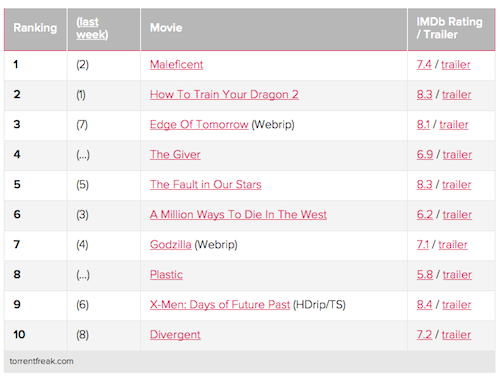
The following shows old/new methods for extracting a table from a web site, including how to use either XPath selectors or CSS selectors in rvest calls. To stave of some potential comments: due to the way this table is setup and the need to extract only certain components from the td blocks and elements from tags within the td blocks, a simple readHTMLTable would not suffice.

The old/new approaches are very similar, but I especially like the ability to chain output ala magrittr/dplyr and not having to mentally switch gears to XPath if I’m doing other work targeting the browser (i.e. prepping data for D3).

The code (sans output) is in this gist, and IMO the rvest package is going to make working with web site data so much easier.

library(XML)
library(httr)
library(rvest)
library(magrittr)

# setup connection & grab HTML the "old" way w/httr
freak_get <- GET("http://torrentfreak.com/top-10-most-pirated-movies-of-the-week-130304/")
freak_html <- htmlParse(content(freak_get, as="text"))

# do the same the rvest way, using "html_session" since we may need connection info in some scripts
freak <- html_session("http://torrentfreak.com/top-10-most-pirated-movies-of-the-week-130304/")

# extracting the "old" way with xpathSApply
xpathSApply(freak_html, "//*/td[3]", xmlValue)[1:10]

##  [1] "Silver Linings Playbook "           "The Hobbit: An Unexpected Journey " "Life of Pi (DVDscr/DVDrip)"        
##  [4] "Argo (DVDscr)"                      "Identity Thief "                    "Red Dawn "                         
##  [7] "Rise Of The Guardians (DVDscr)"     "Django Unchained (DVDscr)"          "Lincoln (DVDscr)"                  
## [10] "Zero Dark Thirty "

xpathSApply(freak_html, "//*/td[1]", xmlValue)[2:11]

##  [1] "1"  "2"  "3"  "4"  "5"  "6"  "7"  "8"  "9"  "10"

xpathSApply(freak_html, "//*/td[4]", xmlValue)

##  [1] "7.4 / trailer" "8.2 / trailer" "8.3 / trailer" "8.2 / trailer" "8.2 / trailer" "5.3 / trailer" "7.5 / trailer"
##  [8] "8.8 / trailer" "8.2 / trailer" "7.6 / trailer"

xpathSApply(freak_html, "//*/td[4]/a[contains(@href,'imdb')]", xmlAttrs, "href")

##                                    href                                    href                                    href 
##  "http://www.imdb.com/title/tt1045658/"  "http://www.imdb.com/title/tt0903624/"  "http://www.imdb.com/title/tt0454876/" 
##                                    href                                    href                                    href 
##  "http://www.imdb.com/title/tt1024648/"  "http://www.imdb.com/title/tt2024432/"  "http://www.imdb.com/title/tt1234719/" 
##                                    href                                    href                                    href 
##  "http://www.imdb.com/title/tt1446192/"  "http://www.imdb.com/title/tt1853728/"  "http://www.imdb.com/title/tt0443272/" 
##                                    href 
## "http://www.imdb.com/title/tt1790885/?"

# extracting with rvest + XPath
freak %>% html_nodes(xpath="//*/td[3]") %>% html_text() %>% .[1:10]

##  [1] "Silver Linings Playbook "           "The Hobbit: An Unexpected Journey " "Life of Pi (DVDscr/DVDrip)"        
##  [4] "Argo (DVDscr)"                      "Identity Thief "                    "Red Dawn "                         
##  [7] "Rise Of The Guardians (DVDscr)"     "Django Unchained (DVDscr)"          "Lincoln (DVDscr)"                  
## [10] "Zero Dark Thirty "

freak %>% html_nodes(xpath="//*/td[1]") %>% html_text() %>% .[2:11]

##  [1] "1"  "2"  "3"  "4"  "5"  "6"  "7"  "8"  "9"  "10"

freak %>% html_nodes(xpath="//*/td[4]") %>% html_text() %>% .[1:10]

##  [1] "7.4 / trailer" "8.2 / trailer" "8.3 / trailer" "8.2 / trailer" "8.2 / trailer" "5.3 / trailer" "7.5 / trailer"
##  [8] "8.8 / trailer" "8.2 / trailer" "7.6 / trailer"

freak %>% html_nodes(xpath="//*/td[4]/a[contains(@href,'imdb')]") %>% html_attr("href") %>% .[1:10]

##  [1] "http://www.imdb.com/title/tt1045658/"  "http://www.imdb.com/title/tt0903624/" 
##  [3] "http://www.imdb.com/title/tt0454876/"  "http://www.imdb.com/title/tt1024648/" 
##  [5] "http://www.imdb.com/title/tt2024432/"  "http://www.imdb.com/title/tt1234719/" 
##  [7] "http://www.imdb.com/title/tt1446192/"  "http://www.imdb.com/title/tt1853728/" 
##  [9] "http://www.imdb.com/title/tt0443272/"  "http://www.imdb.com/title/tt1790885/?"

# extracting with rvest + CSS selectors
freak %>% html_nodes("td:nth-child(3)") %>% html_text() %>% .[1:10]

##  [1] "Silver Linings Playbook "           "The Hobbit: An Unexpected Journey " "Life of Pi (DVDscr/DVDrip)"        
##  [4] "Argo (DVDscr)"                      "Identity Thief "                    "Red Dawn "                         
##  [7] "Rise Of The Guardians (DVDscr)"     "Django Unchained (DVDscr)"          "Lincoln (DVDscr)"                  
## [10] "Zero Dark Thirty "

freak %>% html_nodes("td:nth-child(1)") %>% html_text() %>% .[2:11]

##  [1] "1"  "2"  "3"  "4"  "5"  "6"  "7"  "8"  "9"  "10"

freak %>% html_nodes("td:nth-child(4)") %>% html_text() %>% .[1:10]

##  [1] "7.4 / trailer" "8.2 / trailer" "8.3 / trailer" "8.2 / trailer" "8.2 / trailer" "5.3 / trailer" "7.5 / trailer"
##  [8] "8.8 / trailer" "8.2 / trailer" "7.6 / trailer"

freak %>% html_nodes("td:nth-child(4) a[href*='imdb']") %>% html_attr("href") %>% .[1:10]

##  [1] "http://www.imdb.com/title/tt1045658/"  "http://www.imdb.com/title/tt0903624/" 
##  [3] "http://www.imdb.com/title/tt0454876/"  "http://www.imdb.com/title/tt1024648/" 
##  [5] "http://www.imdb.com/title/tt2024432/"  "http://www.imdb.com/title/tt1234719/" 
##  [7] "http://www.imdb.com/title/tt1446192/"  "http://www.imdb.com/title/tt1853728/" 
##  [9] "http://www.imdb.com/title/tt0443272/"  "http://www.imdb.com/title/tt1790885/?"

# building a data frame (which is kinda obvious, but hey)
data.frame(movie=freak %>% html_nodes("td:nth-child(3)") %>% html_text() %>% .[1:10],
           rank=freak %>% html_nodes("td:nth-child(1)") %>% html_text() %>% .[2:11],
           rating=freak %>% html_nodes("td:nth-child(4)") %>% html_text() %>% .[1:10],
           imdb.url=freak %>% html_nodes("td:nth-child(4) a[href*='imdb']") %>% html_attr("href") %>% .[1:10],
           stringsAsFactors=FALSE)

##                                 movie rank        rating                              imdb.url
## 1            Silver Linings Playbook     1 7.4 / trailer  http://www.imdb.com/title/tt1045658/
## 2  The Hobbit: An Unexpected Journey     2 8.2 / trailer  http://www.imdb.com/title/tt0903624/
## 3          Life of Pi (DVDscr/DVDrip)    3 8.3 / trailer  http://www.imdb.com/title/tt0454876/
## 4                       Argo (DVDscr)    4 8.2 / trailer  http://www.imdb.com/title/tt1024648/
## 5                     Identity Thief     5 8.2 / trailer  http://www.imdb.com/title/tt2024432/
## 6                           Red Dawn     6 5.3 / trailer  http://www.imdb.com/title/tt1234719/
## 7      Rise Of The Guardians (DVDscr)    7 7.5 / trailer  http://www.imdb.com/title/tt1446192/
## 8           Django Unchained (DVDscr)    8 8.8 / trailer  http://www.imdb.com/title/tt1853728/
## 9                    Lincoln (DVDscr)    9 8.2 / trailer  http://www.imdb.com/title/tt0443272/
## 10                  Zero Dark Thirty    10 7.6 / trailer http://www.imdb.com/title/tt1790885/?

To leave a comment for the author, please follow the link and comment on his blog: Data Driven Security.

R-bloggers.com offers daily e-mail updates about R news and tutorials on topics such as: visualization (ggplot2, Boxplots, maps, animation), programming (RStudio, Sweave, LaTeX, SQL, Eclipse, git, hadoop, Web Scraping) statistics (regression, PCA, time series, trading) and more...

Applications of R presentations at Dataweek

$
0
0

(This article was first published on Revolutions, and kindly contributed to R-bloggers)

I'm speaking at the DataWeek conference in San Francisco today. My talk follows Skylar Lyon from Accenture — I'm really looking forward to hearing how he uses Revolution R Enterprise with Teradata Database to run R in-database with 400 million rows of data. Update: Here are Skylar's slides.


The slides for my talk on other companies' applications of R are embedded below.


To leave a comment for the author, please follow the link and comment on his blog: Revolutions.

R-bloggers.com offers daily e-mail updates about R news and tutorials on topics such as: visualization (ggplot2, Boxplots, maps, animation), programming (RStudio, Sweave, LaTeX, SQL, Eclipse, git, hadoop, Web Scraping) statistics (regression, PCA, time series, trading) and more...

BCEA 2.1

$
0
0

(This article was first published on Gianluca Baio's blog, and kindly contributed to R-bloggers)
We're about to release the new version of BCEA, which will contain some major changes.

  1. A couple of changes in the basic code that should improve the computational speed. In general, BCEA doesn't really run into troubles because most of the computations are fairly easy. However, there are a couple of parts in which the code wasn't really optimised; Chris Jackson has suggested some small but substantial modifications $-$ for instance using ColMeans instead of apply($cdot$,2,mean)
  2. Andrea has coded a function to compute the cost-effectiveness efficiency frontier, which is kind of cool. Again, the underlying analysis is not necessarily very complicated, but the resulting graph is quite neat and it is informative and useful too.
  3. We've polished the EVPPI functions (again, thanks to Chris who's spotted a couple of blips in the previous version).
I'll mention this changes in my talk at the workshop on "Efficient Methods for Value of Information Calculations". If all goes to plan, we'll release BCEA 2.1 by the end of this week.

To leave a comment for the author, please follow the link and comment on his blog: Gianluca Baio's blog.

R-bloggers.com offers daily e-mail updates about R news and tutorials on topics such as: visualization (ggplot2, Boxplots, maps, animation), programming (RStudio, Sweave, LaTeX, SQL, Eclipse, git, hadoop, Web Scraping) statistics (regression, PCA, time series, trading) and more...

Animated choropleths to visualize mortality rates of children under 5 and gender differences using rMaps

$
0
0

(This article was first published on Adventures in Analytics and Visualization, and kindly contributed to R-bloggers)
This post displays two animated choropleths. One for global mortality rates for children under 5 (per 1000 live births) and the second for the difference in global mortality rates for males and female children under 5 (per 1000). Please click here: http://patilv.com/MortalityUnder5/

To leave a comment for the author, please follow the link and comment on his blog: Adventures in Analytics and Visualization.

R-bloggers.com offers daily e-mail updates about R news and tutorials on topics such as: visualization (ggplot2, Boxplots, maps, animation), programming (RStudio, Sweave, LaTeX, SQL, Eclipse, git, hadoop, Web Scraping) statistics (regression, PCA, time series, trading) and more...

Fun with .Rprofile and customizing R startup

$
0
0

(This article was first published on On the lambda » ROn the lambda, and kindly contributed to R-bloggers)

Over the years, I've meticulously compiled–and version controlled–massive and extensive configuration files for virtually all of my most used utilities, most notably vim, tmux, and zsh.

In fact, one of the only configurable utilities for which I had no special configuration schema was R. This is extremely surprising, given that I use R everyday.

One reason I think that this was the case is because I came to R from using general-purpose programming languages for which there is no provision to configure the language in a way that would actually change results or program output.

I only vaguely knew that .Rprofile was a configuration file that some people used, and that others warned against using, but it never occurred to me to actually use it for myself.

Because I never used it, I developed odd habits and rituals in my interactive R programming including adding "stringsAsFactors=FALSE" to all of my "read.csv" function calls and making frequent calls to the "option()" function.

Since I actually began to use and expand my R configuration, though, I've realized how much I've been missing. I pre-set all my preferred options (saving time) and I've even made provisions for some cool tricks and hacks.

That being said, there's a certain danger in using a custom R profile but we'll talk about how to thwart that later.

The R Startup Process

In the absence of any command-line flags being used, when R starts up, it will "source" (run) the site-wide R startup configuration file/script if it exists. In a fresh install of R, this will rarely exist, but if it does, it will usually be in '/Library/Frameworks/R.framework/Resources/etc/' on OS X, 'C:Program FilesRR-***etc' on Windows, or '/etc/R/' on Debian. Next, it will check for a .Rprofile hidden file in the current working directory (the directory where R is started on the command-line) to source. Failing that, it will check your home directory for the .Rprofile hidden file.

You can check if you have a site-wide R configuration script by running

R.home(component = "home")

in the R console and then checking for the presence of Rprofile.site in that directory. The presence of the user-defined R configuration can be checked for in the directory of whichever path

path.expand("~")

indicates.

More information on the R startup process can be found here and here.

The site-wide R configuration script
For most R installations on primarily single-user systems, using the site-wide R configuration script should be given up in favor of the user-specific configuration. That being said, a look at the boilerplate site-wide R profile that Debian furnishes (but comments out by default) provides some good insight into what might be a good idea to include in this file, if you choose to use it.

##                      Emacs please make this -*- R -*-
## empty Rprofile.site for R on Debian
##
## Copyright (C) 2008 Dirk Eddelbuettel and GPL'ed
##
## see help(Startup) for documentation on ~/.Rprofile and Rprofile.site

# ## Example of .Rprofile
# options(width=65, digits=5)
# options(show.signif.stars=FALSE)
# setHook(packageEvent("grDevices", "onLoad"),
#         function(...) grDevices::ps.options(horizontal=FALSE))
# set.seed(1234)
# .First <- function() cat("n   Welcome to R!nn")
# .Last <- function()  cat("n   Goodbye!nn")

# ## Example of Rprofile.site
# local({
#  # add MASS to the default packages, set a CRAN mirror
#  old <- getOption("defaultPackages"); r <- getOption("repos")
#  r["CRAN"] <- "http://my.local.cran"
#  options(defaultPackages = c(old, "MASS"), repos = r)
#})

Two things you might want to do in a site-wide R configuration file is add other packages to the default packages list and set a preferred CRAN mirror. Other things that the above snippet indicates you can do is set various width and number display options, setting a random-number seed (making random number generation deterministic for reproducible analysis), and hiding the stars that R shows for different significance levels (ostensibly because of their connection to the much-maligned NHST paradigm).

The user-specific .Rprofile
In contrast to the site-wide config (that will be used for all users on the system), the user-specific R configuration file is a place to put more personal preferences, shortcuts, aliases, and hacks. Immediately below is my .Rprofile.

local({r <- getOption("repos")
      r["CRAN"] <- "http://cran.revolutionanalytics.com"
      options(repos=r)})

options(stringsAsFactors=FALSE)

options(max.print=100)

options(scipen=10)

options(editor="vim")

# options(show.signif.stars=FALSE)

options(menu.graphics=FALSE)

options(prompt="> ")
options(continue="... ")

options(width = 80)

q <- function (save="no", ...) {
  quit(save=save, ...)
}

utils::rc.settings(ipck=TRUE)

.First <- function(){
  if(interactive()){
    library(utils)
    timestamp(,prefix=paste("##------ [",getwd(),"] ",sep=""))

  }
}

.Last <- function(){
  if(interactive()){
    hist_file <- Sys.getenv("R_HISTFILE")
    if(hist_file=="") hist_file <- "~/.RHistory"
    savehistory(hist_file)
  }
}

if(Sys.getenv("TERM") == "xterm-256color")
  library("colorout")

sshhh <- function(a.package){
  suppressWarnings(suppressPackageStartupMessages(
    library(a.package, character.only=TRUE)))
}

auto.loads <-c("dplyr", "ggplot2")

if(interactive()){
  invisible(sapply(auto.loads, sshhh))
}

.env <- new.env()
attach(.env)

.env$unrowname <- function(x) {
  rownames(x) <- NULL
  x
}

.env$unfactor <- function(df){
  id <- sapply(df, is.factor)
  df[id] <- lapply(df[id], as.character)
  df
}

message("n*** Successfully loaded .Rprofile ***n")

[Lines 1-3]: First, because I don't have a site-wide R configuration script, I set my local CRAN mirror here. My particular choice of mirror is largely arbitrary.

[Line 5]: If stringsAsFactors hasn't bitten you yet, it will.

[Line 9]: Setting 'scipen=10' effectively forces R to never use scientific notation to express very small or large numbers.

[Line 13]: I included the snippet to turn off significance stars because it is a popular choice, but I have it commented out because ever since 1st grade I've used number of stars as a proxy for my worth as a person.

[Line 15]: I don't have time for Tk to load; I'd prefer to use the console, if possible.

[Lines 17-18]: Often, when working in the interactive console I forget a closing brace or paren. When I start a new line, R changes the prompt to "+" to indicate that it is expecting a continuation. Because "+" and ">" are the same width, though, I often don't notice and really screw things up. These two lines make the R REPL mimic the Python REPL by changing the continuation prompt to the wider "...".

[Lines 22-24]: Change the default behavior of "q()" to quit immediately and not save workspace.

[Line 26]: This snippet allows you to tab-complete package names for use in "library()" or "require()" calls. Credit for this one goes to @mikelove.

[Lines 28-34]: There are three main reasons I like to have R save every command I run in the console into a history file.

  • Occasionally I come up with a clever way to solve a problem in an interactive session that I may want to remember for later use; instead of it getting lost in the ether, if I save it to a history file, I can look it up later.
  • Sometimes I need an alibi for what I was doing at a particular time
  • I ran a bunch of commands in the console to perform an analysis not realizing that I would have to repeat this analysis later. I can retrieve the commands from a history file and put it into a script where it belongs.

These lines instruct R to, before anything else, echo a timestamp to the console and to my R history file. The timestamp greatly improves my ability to search through my history for relevant commands.

[Lines 36-42]: These lines instruct R, right before exiting, to write all commands I used in that session to my R command history file. I usually have this set in an environment variable called "R_HISTFILE" on most of my systems, but in case I don't have this defined, I write it to a file in my home directory called .Rhistory.

[Line 44]: Enables the colorized output from R (provided by the colorout package) on appropriate consoles.

[Lines 47-50]: This defines a function that loads a libary into the namespace without any warning or startup messages clobbering my console.

[Line 52]: I often want to autoload the 'dplyr' and 'ggplot2' packages (particularly 'dplyr' as it is now an integral part of my R experience).

[Lines 54-56]: This loads the packages in my "auto.loads" vector if the R session is interactive.

[Lines 58-59]: This creates a new hidden namespace that we can store some functions in. We need to do this in order for these functions to survive a call to "rm(list=ls())" which will remove everything in the current namespace. This is described wonderfully in this blog post.

[Lines 61-64]: This defines a simple function to remove any row names a data.frame might have. This was stolen from Stephen Turner (which was in turn stolen from plyr).

[Lines 66-70]: This defines a function to sanely undo a "factor()" call. This was stolen from Dason Kurkiewicz.

Warnings about .Rprofile
There are some compelling reasons to abstain from using an R configuration file at all. The most persuasive argument against using it is the portability issue: As you begin to rely more and more on shortcuts and options you define in your .Rprofile, your R scripts will depend on them more and more. If a script is then transferred to a friend or colleague, often it won't work; in the worst case scenario, it will run without error but produce wrong results.

There are several ways this pitfall can be avoided, though:

  • For R sessions/scripts that might be shared or used on systems without your .Rprofile, make sure to start the R interpreter with the --vanilla option, or add/change your shebang lines to "#!/usr/bin/Rscript --vanilla". The "--vanilla" option will tell R to ignore any configuration files. Writing scripts that will conform to a vanilla R startup environment is a great thing to do for portability.
  • Use your .Rprofile everywhere! This is a bit of an untenable solution because you can't put your .Rprofile everywhere. However, if you put your .Rprofile on GitHub, you can easily clone it on any system that needs it. You can find mine here.
  • Save your .Rprofile to another file name and, at the start of every R session where you want to use your custom configuration, manually source the file. This will behave just as it would if it were automatically sourced by R but removes the potential for the .Rprofile to be sourced when it is unwanted.

    A variation on this theme is to create a shell alias to use R with your special configuration. For example, adding a shell alias like this:

    alias aR="R_PROFILE_USER=~/.myR/aR.profile R"
    

    will make it so that when "R" is run, it will run as before (without special configuration). In order to have R startup and auto-source your configuration you now have to run "aR". When 'aR' is run, the shell temporarily assigns an environment variable that R will follow to source a config script. In this case, it will source a config file called aR.profile in a hidden .myR subdirectory of my home folder. This path can be changed to anything, though.

This is the solution I have settled on because it is very easy to live with and invalidates concerns about portability.

share this: facebooktwittergoogle_plusredditpinterestlinkedintumblrmail

To leave a comment for the author, please follow the link and comment on his blog: On the lambda » ROn the lambda.

R-bloggers.com offers daily e-mail updates about R news and tutorials on topics such as: visualization (ggplot2, Boxplots, maps, animation), programming (RStudio, Sweave, LaTeX, SQL, Eclipse, git, hadoop, Web Scraping) statistics (regression, PCA, time series, trading) and more...

Space Invaders

$
0
0

(This article was first published on Ripples, and kindly contributed to R-bloggers)

I burned through all of my extra lives in a matter of minutes, and my two least-favorite words appeared on the screen: GAME OVER (Ernest Cline, Ready Player One)

Inspired by the book I read this summer and by this previous post, I decided to draw these aliens:

Invader1 Invader3
Invader4Invader2

Do not miss to check this indispensable document to choose your favorite colors:

require("ggplot2")
require("reshape")
mars1=matrix(c(0,0,0,0,0,0,0,0,0,0,0,0,
0,0,0,1,0,0,0,0,1,0,0,0,
0,0,0,0,1,0,0,1,0,0,0,0,
0,0,0,1,1,1,1,1,1,0,0,0,
0,0,1,1,0,1,1,0,1,1,0,0,
0,1,1,1,1,1,1,1,1,1,1,0,
0,1,1,1,1,1,1,1,1,1,1,0,
0,1,1,1,1,1,1,1,1,1,1,0,
0,1,1,1,1,1,1,1,1,1,1,0,
0,1,0,1,0,0,0,0,1,0,1,0,
0,1,0,0,1,0,0,1,0,0,1,0,
0,0,0,0,0,0,0,0,0,0,0,0), nrow=12, byrow = TRUE)
mars2=matrix(c(0,0,0,0,0,0,0,0,0,0,0,0,
0,0,0,0,0,1,1,0,0,0,0,0,
0,0,0,0,1,1,1,1,0,0,0,0,
0,0,0,1,1,1,1,1,1,0,0,0,
0,0,1,1,0,1,1,0,1,1,0,0,
0,1,1,1,1,1,1,1,1,1,1,0,
0,1,1,1,1,1,1,1,1,1,1,0,
0,0,0,0,1,0,0,1,0,0,0,0,
0,0,0,1,0,1,1,0,1,0,0,0,
0,0,1,0,1,0,0,1,0,1,0,0,
0,1,0,1,0,0,0,0,1,0,1,0,
0,0,0,0,0,0,0,0,0,0,0,0), nrow=12, byrow = TRUE)
mars3=matrix(c(0,0,0,0,0,0,0,0,0,0,0,0,
0,0,0,0,1,0,0,1,0,0,0,0,
0,0,0,1,0,0,0,0,1,0,0,0,
0,0,0,1,1,1,1,1,1,0,0,0,
0,0,1,1,0,1,1,0,1,1,0,0,
0,1,1,1,1,1,1,1,1,1,1,0,
0,1,1,1,1,1,1,1,1,1,1,0,
0,1,1,1,1,1,1,1,1,1,1,0,
0,1,0,1,0,0,0,0,1,0,1,0,
0,1,0,0,1,1,1,1,0,0,1,0,
0,0,0,0,1,0,0,1,0,0,0,0,
0,0,0,0,0,0,0,0,0,0,0,0), nrow=12, byrow = TRUE)
mars4=matrix(c(0,0,0,0,0,0,0,0,0,0,0,0,
0,0,0,0,0,1,1,0,0,0,0,0,
0,0,0,0,1,1,1,1,0,0,0,0,
0,0,0,1,1,1,1,1,1,0,0,0,
0,0,1,1,0,1,1,0,1,1,0,0,
0,1,1,1,1,1,1,1,1,1,1,0,
0,1,1,1,1,1,1,1,1,1,1,0,
0,1,0,0,1,0,0,1,0,0,1,0,
0,0,0,1,0,0,0,0,1,0,0,0,
0,0,0,0,1,0,0,1,0,0,0,0,
0,0,0,1,0,0,0,0,1,0,0,0,
0,0,0,0,0,0,0,0,0,0,0,0), nrow=12, byrow = TRUE)
opt=theme(legend.position="none",
panel.background = element_blank(),
panel.grid = element_blank(),
axis.ticks = element_blank(),
axis.title = element_blank(),
axis.text = element_blank())
p1=ggplot(melt(mars1), aes(x=X2, y=X1))+geom_tile(aes(fill=jitter(value, amount=.1)), colour="gray65", lwd=.025)+
scale_fill_gradientn(colours = c("chartreuse", "navy"))+scale_y_reverse()+opt
p2=ggplot(melt(mars2), aes(x=X2, y=X1))+geom_tile(aes(fill=jitter(value, amount=.1)), colour="gray65", lwd=.025)+
scale_fill_gradientn(colours = c("olivedrab1", "magenta4"))+scale_y_reverse()+opt
p3=ggplot(melt(mars3), aes(x=X2, y=X1))+geom_tile(aes(fill=jitter(value, amount=.1)), colour="gray65", lwd=.025)+
scale_fill_gradientn(colours = c("violetred4", "yellow"))+scale_y_reverse()+opt
p4=ggplot(melt(mars4), aes(x=X2, y=X1))+geom_tile(aes(fill=jitter(value, amount=.1)), colour="gray65", lwd=.025)+
scale_fill_gradientn(colours = c("tomato4", "lawngreen"))+scale_y_reverse()+opt

To leave a comment for the author, please follow the link and comment on his blog: Ripples.

R-bloggers.com offers daily e-mail updates about R news and tutorials on topics such as: visualization (ggplot2, Boxplots, maps, animation), programming (RStudio, Sweave, LaTeX, SQL, Eclipse, git, hadoop, Web Scraping) statistics (regression, PCA, time series, trading) and more...

Stay on track: Plotting GPS tracks with R

$
0
0

(This article was first published on Rcrastinate, and kindly contributed to R-bloggers)
Many GPS devices and apps have the capability to track your current position via GPS. If you go walking, running, cycling, flying or driving, you can take a look at your exact route and your average speed.

Some of these devices or apps also allow you to export your routes in various formats, e.g., the popular XML-based GPX format.

I want to show you my attempts to
- read in a GPX file using R and its XML package,
- calculate distances and speeds between points,
- plot elevation and speed,
- plot a track,
- plot a track on a map.

Here are the results. Everything below the plots shows you how to do it in R. Drop me a comment if you have any questions.


The altitude of the track in time, with smoother. Click to enlarge.

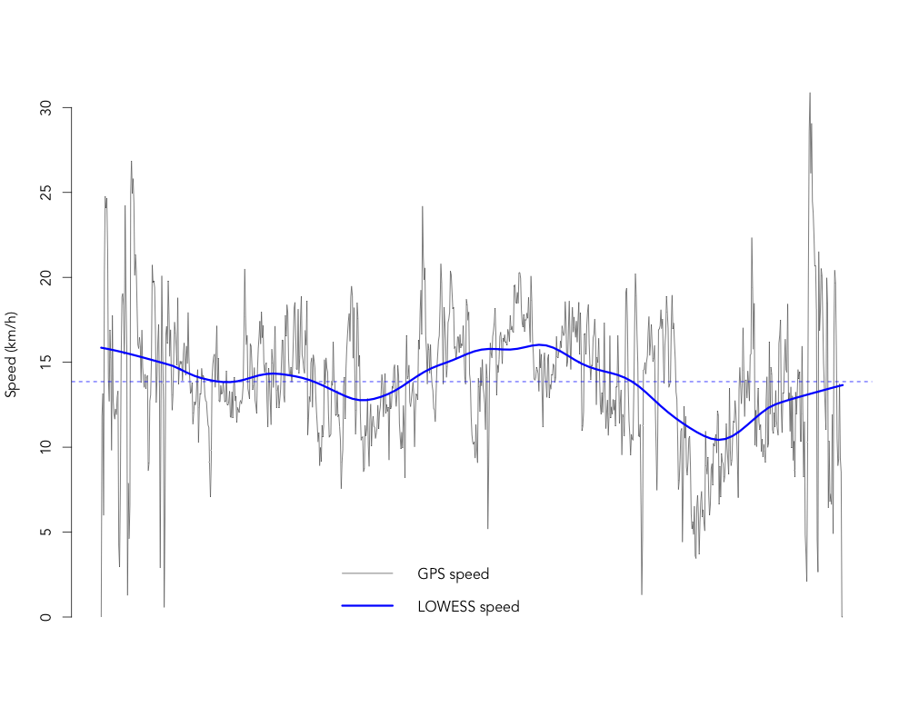
The speed during the run, with smoother. Click to enlarge.

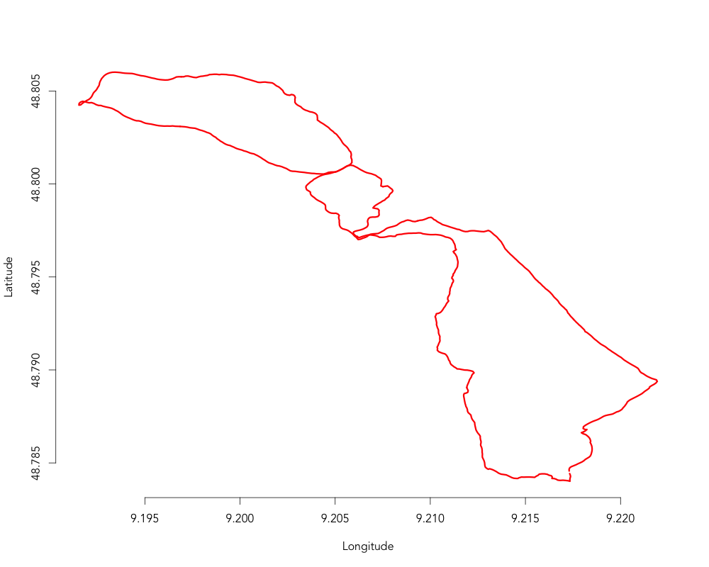
The raw track without a map in the background. Click to enlarge.

The track with an OpenStreetMap of Stuttgart in the background.

The track with a Bing map of Stuttgart in the background. Click to enlarge.

The track with a Mapquest map of Stuttgart in the background. Click to enlarge.

Again the same track, now with Skobbler map of Stuttgart in the background. Click to enlarge.


If you want to replicate this script, you can use an example GPX file I uploaded. It's one of my runs through Stuttgart. The file name is "run.gpx".

We gonna need some packages.

library(XML)
library(OpenStreetMap)
library(lubridate)

And a function that shifts vectors conviniently (we gonna need this later):

shift.vec <- function (vec, shift) {
  if(length(vec) <= abs(shift)) {
    rep(NA ,length(vec))
  }else{
    if (shift >= 0) {
      c(rep(NA, shift), vec[1:(length(vec)-shift)]) }
    else {
      c(vec[(abs(shift)+1):length(vec)], rep(NA, abs(shift))) } } }

Now, we're reading in the GPX file. If you want help on parsing XML files, check out this (German) tutorial I made a while ago.

# Parse the GPX file
pfile <- htmlTreeParse("run.gpx",
                      error = function (...) {}, useInternalNodes = T)
# Get all elevations, times and coordinates via the respective xpath
elevations <- as.numeric(xpathSApply(pfile, path = "//trkpt/ele", xmlValue))
times <- xpathSApply(pfile, path = "//trkpt/time", xmlValue)
coords <- xpathSApply(pfile, path = "//trkpt", xmlAttrs)
# Extract latitude and longitude from the coordinates
lats <- as.numeric(coords["lat",])
lons <- as.numeric(coords["lon",])
# Put everything in a dataframe and get rid of old variables
geodf <- data.frame(lat = lats, lon = lons, ele = elevations, time = times)
rm(list=c("elevations", "lats", "lons", "pfile", "times", "coords"))
head(geodf)
       lat      lon ele                   time
1 48.78457 9.217300 312 2014-08-17T17:25:07.45
2 48.78457 9.217300 312 2014-08-17T17:25:07.52
3 48.78466 9.217295 311 2014-08-17T17:25:10.53
4 48.78475 9.217335 307 2014-08-17T17:25:13.50
5 48.78480 9.217410 310 2014-08-17T17:25:19.51
6 48.78486 9.217550 306 2014-08-17T17:25:22.49

We already have nice dataframe now with all the information available in the GPX file for each position. Each position is defined by the latitude and longitude and we also have the elevation (altitude) available. Note, that the altitude ist quite noisy with GPS, we will see this in a minute.

Now, let's calculate the distances between successive positions and the respective speed in this segment.

# Shift vectors for lat and lon so that each row also contains the next position.
geodf$lat.p1 <- shift.vec(geodf$lat, -1)
geodf$lon.p1 <- shift.vec(geodf$lon, -1)
# Calculate distances (in metres) using the function pointDistance from the 'raster' package.
# Parameter 'lonlat' has to be TRUE!
geodf$dist.to.prev <- apply(geodf, 1, FUN = function (row) {
  pointDistance(c(as.numeric(row["lat.p1"]),
  as.numeric(row["lon.p1"])),
                c(as.numeric(row["lat"]), as.numeric(row["lon"])),
                lonlat = T)
})
# Transform the column 'time' so that R knows how to interpret it.
geodf$time <- strptime(geodf$time, format = "%Y-%m-%dT%H:%M:%OS")
# Shift the time vector, too.
geodf$time.p1 <- shift.vec(geodf$time, -1)
# Calculate the number of seconds between two positions.
geodf$time.diff.to.prev <- as.numeric(difftime(geodf$time.p1, geodf$time))
# Calculate metres per seconds, kilometres per hour and two LOWESS smoothers to get rid of some noise.
geodf$speed.m.per.sec <- geodf$dist.to.prev / geodf$time.diff.to.prev
geodf$speed.km.per.h <- geodf$speed.m.per.sec * 3.6
geodf$speed.km.per.h <- ifelse(is.na(geodf$speed.km.per.h), 0, geodf$speed.km.per.h)
geodf$lowess.speed <- lowess(geodf$speed.km.per.h, f = 0.2)$y
geodf$lowess.ele <- lowess(geodf$ele, f = 0.2)$y

Now, let's plot all the stuff!

# Plot elevations and smoother
plot(geodf$ele, type = "l", bty = "n", xaxt = "n", ylab = "Elevation", xlab = "", col = "grey40")
lines(geodf$lowess.ele, col = "red", lwd = 3)
legend(x="bottomright", legend = c("GPS elevation", "LOWESS elevation"),
       col = c("grey40", "red"), lwd = c(1,3), bty = "n")

# Plot speeds and smoother
plot(geodf$speed.km.per.h, type = "l", bty = "n", xaxt = "n", ylab = "Speed (km/h)", xlab = "",
     col = "grey40")
lines(geodf$lowess.speed, col = "blue", lwd = 3)
legend(x="bottom", legend = c("GPS speed", "LOWESS speed"),
       col = c("grey40", "blue"), lwd = c(1,3), bty = "n")
abline(h = mean(geodf$speed.km.per.h), lty = 2, col = "blue")

# Plot the track without any map, the shape of the track is already visible.
plot(rev(geodf$lon), rev(geodf$lat), type = "l", col = "red", lwd = 3, bty = "n", ylab = "Latitude", xlab = "Longitude")

We will now use the OpenStreetMap package to get some maps from the internet and use them as a background for the track we just converted. There are several blocks for each map type. Check the comments in the first block what the different calls do.

First, we need to get the specific map. The 'type' argument controls which type of map we get.

map <- openmap(as.numeric(c(max(geodf$lat), min(geodf$lon))),
               as.numeric(c(min(geodf$lat), max(geodf$lon))), type = "osm")

This next step is important and it took me a while to figure this out. We need to convert the maps we got with the function openmap() to a projection that fits our longitude-latitude format of positions. This will distort the maps in the plots a little. But we need this step because the track has to fit the map!

transmap <- openproj(map, projection = "+proj=longlat")

# Now for plotting...
png("map1.png", width = 1000, height = 800, res = 100)
par(mar = rep(0,4))
plot(transmap, raster=T)
lines(geodf$lon, geodf$lat, type = "l", col = scales::alpha("red", .5), lwd = 4)
dev.off()

map <- openmap(as.numeric(c(max(geodf$lat), min(geodf$lon))),
               as.numeric(c(min(geodf$lat), max(geodf$lon))), type = "bing")

transmap <- openproj(map, projection = "+proj=longlat")
png("map2.png", width = 1000, height = 800, res = 100)
par(mar = rep(0,4))
plot(transmap, raster=T)
lines(geodf$lon, geodf$lat, type = "l", col = scales::alpha("yellow", .5), lwd = 4)
dev.off()

map <- openmap(as.numeric(c(max(geodf$lat), min(geodf$lon))),
               as.numeric(c(min(geodf$lat), max(geodf$lon))), type = "mapquest")

transmap <- openproj(map, projection = "+proj=longlat")
png("map3.png", width = 1000, height = 800, res = 100)
par(mar = rep(0,4))
plot(transmap, raster=T)
lines(geodf$lon, geodf$lat, type = "l", col = scales::alpha("yellow", .5), lwd = 4)
dev.off()

map <- openmap(as.numeric(c(max(geodf$lat), min(geodf$lon))),
               as.numeric(c(min(geodf$lat), max(geodf$lon))), type = "skobbler")

transmap <- openproj(map, projection = "+proj=longlat")
png("map4.png", width = 1000, height = 800, res = 100)
par(mar = rep(0,4))
plot(transmap, raster=T)
lines(geodf$lon, geodf$lat, type = "l", col = scales::alpha("blue", .5), lwd = 4)
dev.off()

map <- openmap(as.numeric(c(max(geodf$lat), min(geodf$lon))),
               as.numeric(c(min(geodf$lat), max(geodf$lon))), type = "esri-topo")

transmap <- openproj(map, projection = "+proj=longlat")
png("map5.png", width = 1000, height = 800, res = 100)
par(mar = rep(0,4))
plot(transmap, raster=T)
lines(geodf$lon, geodf$lat, type = "l", col = scales::alpha("blue", .5), lwd = 4)
dev.off()

To leave a comment for the author, please follow the link and comment on his blog: Rcrastinate.

R-bloggers.com offers daily e-mail updates about R news and tutorials on topics such as: visualization (ggplot2, Boxplots, maps, animation), programming (RStudio, Sweave, LaTeX, SQL, Eclipse, git, hadoop, Web Scraping) statistics (regression, PCA, time series, trading) and more...

Comparing machine learning models in R

$
0
0

(This article was first published on Revolutions, and kindly contributed to R-bloggers)

by Joseph Rickert

While preparing for the DataWeek R Bootcamp that I conducted this week I came across the following gem. This code, based directly on a Max Kuhn presentation of a couple years back, compares the efficacy of two machine learning models on a training data set.

#-----------------------------------------
# SET UP THE PARAMETER SPACE SEARCH GRID
ctrl <- trainControl(method="repeatedcv",	        # use repeated 10fold cross validation
		     repeats=5,	                        # do 5 repititions of 10-fold cv
		     summaryFunction=twoClassSummary,	# Use AUC to pick the best model
		     classProbs=TRUE)
# Note that the default search grid selects 3 values of each tuning parameter
#
grid <- expand.grid(.interaction.depth = seq(1,7,by=2), # look at tree depths from 1 to 7
		    .n.trees=seq(10,100,by=5),	        # let iterations go from 10 to 100
		    .shrinkage=c(0.01,0.1))		# Try 2 values of the learning rate parameter
 
# BOOSTED TREE MODEL										
set.seed(1)
names(trainData)
trainX <-trainData[,4:61]
 
registerDoParallel(4)		                        # Registrer a parallel backend for train
getDoParWorkers()
 
system.time(gbm.tune <- train(x=trainX,y=trainData$Class,
				method = "gbm",
				metric = "ROC",
				trControl = ctrl,
				tuneGrid=grid,
				verbose=FALSE))
 
#---------------------------------
# SUPPORT VECTOR MACHINE MODEL
#
set.seed(1)
registerDoParallel(4,cores=4)
getDoParWorkers()
system.time(
	svm.tune <- train(x=trainX, y= trainData$Class,
				method = "svmRadial",
				tuneLength = 9,		# 9 values of the cost function
				preProc = c("center","scale"),
				metric="ROC",
				trControl=ctrl)	        # same as for gbm above
)	
#-----------------------------------
# COMPARE MODELS USING RESAPMLING
# Having set the seed to 1 before running gbm.tune and svm.tune we have generated paired samplesfor comparing models using resampling.
#
# The resamples function in caret collates the resampling results from the two models
rValues <- resamples(list(svm=svm.tune,gbm=gbm.tune))
rValues$values
#---------------------------------------------
# BOXPLOTS COMPARING RESULTS
bwplot(rValues,metric="ROC")		# boxplot

After setting up a grid to search the parameter space of a model, the train() function from the caret package is used used to train a generalized boosted regression model (gbm) and a support vector machine (svm). Setting the seed produces paired samples and enables the two models to be compared using the resampling technique described in Hothorn at al, "The design and analysis of benchmark experiments", Journal of Computational and Graphical Statistics (2005) vol 14 (3) pp 675-699

The performance metric for the comparison is the ROC curve. From examing the boxplots of the sampling distributions for the two models it is apparent that, in this case, the gbm has the advantage.

Svm_gbm_boxes

Also, notice that the call to registerDoParallel() permits parallel execution of the training algorithms. (The taksbar showed all foru cores of my laptop maxed out at 100% utilization.)

I chose this example because I wanted to show programmers coming to R for the first time that the power and productivity of R comes not only from the large number of machine learning models implemented, but also from the tremendous amount of infrastructure that package authors have built up, making it relatively easy to do fairly sophisticated tasks in just a few lines of code.

All of the code for this example along with the rest of the my code from the Datweek R Bootcamp is available on GitHub.

To leave a comment for the author, please follow the link and comment on his blog: Revolutions.

R-bloggers.com offers daily e-mail updates about R news and tutorials on topics such as: visualization (ggplot2, Boxplots, maps, animation), programming (RStudio, Sweave, LaTeX, SQL, Eclipse, git, hadoop, Web Scraping) statistics (regression, PCA, time series, trading) and more...

Interactive Visualizations from R using rCharts

$
0
0

(This article was first published on Data Science Los Angeles » R, and kindly contributed to R-bloggers)

At useR! 2014 Ramnath Vaidyanathan gave a tutorial and a presentation on one of his current project, rCharts. This R package allows you to create, customize and share interactive visualizations straight from R. rCharts leverages several existing javascript visualization libraries such as polychart, MorrisJS, NVD3, xCharts, HighCharts, leaflet, and Rickshaw, providing R users a fantastic array of new features and visualization styles.

rCharts also provides a convenient method to share these charts, either in standalone mode, by using a Shiny application, or even in a blog post using knitR! Continuing with the theme of the conference of R as an interface, Ramnath has succeeded in creating a powerful system to smoothly move between the familiar lattice plotting interface and the best available visualization libraries.

In this talk, Ramnath provides a high level overview of rCharts, as well as providing a deep dive into the kinds of visualizations possible with this tool – including the interactive visualizations now at your fingertips. From barcharts to mapping, from static to interactive, Ramnath covers many common use cases with this package, and we encourage you to follow along with the video below using his provided slides from the original talk. Enjoy!

To leave a comment for the author, please follow the link and comment on his blog: Data Science Los Angeles » R.

R-bloggers.com offers daily e-mail updates about R news and tutorials on topics such as: visualization (ggplot2, Boxplots, maps, animation), programming (RStudio, Sweave, LaTeX, SQL, Eclipse, git, hadoop, Web Scraping) statistics (regression, PCA, time series, trading) and more...

“Do You Want to Steal a Snowman?” – A Look (with R) At TorrentFreak’s Top 10 PiRated Movies List #TLAPD

$
0
0

(This article was first published on Data Driven Security, and kindly contributed to R-bloggers)

img

We leave the Jolly Roger behind this year and turn our piRate spyglass towards the digital seas and take a look at piRated movies as seen through the lens of TorrentFreak. The seasoned seadogs who pilot that ship have been doing a weekly “Top 10 Pirated Movies of the Week” post since early 2013, and I thought it might be fun to gather, process, analyze and visualize the data for this year’s annual TLAPD post. So, let’s weigh anchor and set sail!

NOTE: I’m leaving out some cruft from this post - such as all the library() calls - and making use of comments in code snippets to help streamline the already quite long presentaiton. You can grab all the code+data over at it’s github repo. It will be much easier to run the R project code from there.

Since this is a code-heavy post, you’ve got the option to toggle the code segments for readability. Remember, too, that all lightbox-displayed images can be right-clicked/saved-as (or open tabbed) for full scale viewing.

PlundeRing the PiRate Data

To do any kind of analysis & visualization you need data (#CaptainObvious). While TorrentFreak has an RSS feed for their “top 10”, I haven’t been a subscriber to it, so needed to do some piRating of my own to get some data to work with. After inspecting their top 10 posts, I discovered that they used plain ol’ HTML <table>‘s for markup (which, thankfully, was very uniformly applied across the posts).

R excels at scraping data from the web, and I was able to use the new rvest package to grab the pages and extract the table contents. The function below iterates over every week since March 3, 2013, grabs the table from the page and stores it in a data frame. Note that there are two different formats for the URLs (I suspect that indicates multiple authors with their own personal standards for article slugs) that need to be handled by the function:

scrapeMovieData <- function() {

  # get all the Mondays (which is when torrentfreak does their top 10 post)
  # they seem to have started on March 3rd and the URL format varies slightly

  dates <- seq.Date(as.Date("2013-03-03"), as.Date("2014-09-17"), by="1 day")
  mondays <- format(dates[weekdays(dates)=="Monday"], "%y%m%d")

  # pblapply gives us progress bars for free!

  do.call("rbind", pblapply(mondays, function(day) {

    freak <- html_session(sprintf("http://torrentfreak.com/top-10-most-pirated-movies-of-the-week-%s/", day))
    if (freak$response$status_code >= 400) {
      freak <- html_session(sprintf("http://torrentfreak.com/top-10-pirated-movies-week-%s/", day))
    }

    data.frame(date=as.Date(day, format="%y%m%d")-1,
               movie=freak %>% html_nodes("td:nth-child(3)") %>% html_text() %>% .[1:10],
               rank=freak %>% html_nodes("td:nth-child(1)") %>% html_text() %>% .[2:11],
               rating=freak %>% html_nodes("td:nth-child(4)") %>% html_text() %>% .[1:10],
               imdb.url=freak %>% html_nodes("td:nth-child(4) a[href*='imdb']") %>% html_attr("href") %>% .[1:10],
               stringsAsFactors=FALSE)

  }))

}

If you’re trying this from your Captain’s quarters, you’ll see the use of pblapply which is a great way to get a progress bar with almost no effort. A progress bar is somewhat necessary since it can take a little while to grab all this data. If you look at the entire R script on github, you’ll see that it doesn’t scrape this data every time it’s run. It looks for an existing serialized RData file before kicking off the web requests. This saves TorrentFreak (and you) some bandwidth. This process can further be optimized to allow for future scraping of only new data (i.e. use an rda file as a cache.)

TorrentFreak records:

  • PiRate Rank that week (i.e. most downloads to least downloads)
  • PiRate Rank the previous week (which we won’t be using)
  • The Movie Title (often with a link to the Rotten Tomatoes page for it)
  • The IMDb Rating (if there is one) and a link to the IMDb page for the movie
  • A link to the trailer (which we won’t be using)

After the download step, we’re left with a data frame that is still far from shipshape. Many of the titles have annotations (e.g. “Captain America: The Winter Soldier (Cam/TS)“) indicating the source material type. Some titles have…interesting…encodings. There are leading and trailing blanks in some of the titles. The titles aren’t capitalized consistently or use numbers instead of Roman numerals (it turns out this isn’t too important to fix as we’ll see later). The IMDb rating needs cleaning up, and there are other bits that need some twiddling.

In the spirit of Reproducible ReseaRch (and to avoid having to “remember” what one did in a text editor to clean up a file) a cleanup function like the one below is extrememly valuable. The data can be regenerated at any time (provided it’s still scrapeable, though you could archive full pages as well) and the function can be modified when some new condition arises (in this case some new “rip types” appeared over the course of preparing this post).

cleanUpMovieData <- function(imdb) {

  # all of this work on the title is prbly not necessary since we just end up using the 
  # normalized Title field from the OMDb; but, I did this first so I'm keeping it in.
  # goshdarnit

  # handle encodings & leading/trailing blanks
  imdb$movie <- gsub("^ +| +$", "", iconv(imdb$movie, to="UTF-8"))

  # stupid factors get in the way sometimes so convert them all!
  imdb[] <- lapply(imdb, as.character)

  # eliminate the "rip types"
  imdb$movie <- gsub(" * \((Camaudio|Cam audio|CAM|Cam|CAM/R5|CAM/TS|Cam/TS|DVDscr|DVDscr/BrRip|DVDscr/DVDrip|HDCAM|HDTS|R6|R6/CAM|R6/Cam|R6/TS|TS|TS/Cam|TS/Webrip|Webrip|Webrip/TS|HDrip/TS)\)", "", imdb$movie, ignore.case=TRUE)

  # normalize case & punctuation, though some of this isn't really necessary since
  # we have the IMDB id and can get the actual "real" title that way, but this is
  # an OK step if we didn't have that other API to work with (and didn't during the
  # initial building of the example)

  imdb$movie <- gsub("’", "'", imdb$movie)
  imdb$movie <- gsub(" a ", " a ", imdb$movie, ignore.case=TRUE)
  imdb$movie <- gsub(" of ", " of ", imdb$movie, ignore.case=TRUE)
  imdb$movie <- gsub(" an ", " an ", imdb$movie, ignore.case=TRUE)
  imdb$movie <- gsub(" and ", " and ", imdb$movie, ignore.case=TRUE)
  imdb$movie <- gsub(" is ", " is ", imdb$movie, ignore.case=TRUE)
  imdb$movie <- gsub(" the ", " the ", imdb$movie, ignore.case=TRUE)
  imdb$movie <- gsub("Kick Ass", "Kick-Ass", imdb$movie, fixed=TRUE)
  imdb$movie <- gsub("Part III", "Part 3", imdb$movie, fixed=TRUE)
  imdb$movie <- gsub("\:", "", imdb$movie)
  imdb$movie <- gsub(" +", " ", imdb$movie)

  # the IMDB rating is sometimes wonky
  imdb$rating <- gsub(" /.*$", "", imdb$rating)
  imdb$rating <- gsub("?.?", NA, imdb$rating, fixed=TRUE)
  imdb$rating <- as.numeric(imdb$rating)

  # need some things numeric and as dates
  imdb$rank <- as.numeric(imdb$rank)

  imdb$date <- as.Date(imdb$date)

  # extract the IMDb title code
  imdb$imdb.url <- str_extract(imdb$imdb.url, "(tt[0-9]+)")

  # use decent column names efficiently thanks to data.table
  setnames(imdb, colnames(imdb), c("date", "movie", "rank", "rating", "imdb.id"))

  imdb

}

combined <- cleanUpMovieData(scrapeMovieData())

ExploRing the PiRate Data

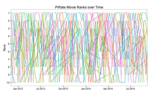
We can take an initial look at this data by plotting the movies by rank over time and using some dplyr idioms (select the picture to see a larger/longer chart):

combined %>%
  select(Title, rank, date) %>%          # only need these fields
  ggplot(aes(x=date, y=rank)) +          # plotting by date & rank
  scale_y_reverse(breaks=c(10:1)) +      # '1' shld be at the top and we want integer labels
  scale_x_date(expand=c(0,0)) +          # tighten the x axis margins
  geom_line(aes(color=Title)) +          # plot the lines
  labs(x="", y="Rank", title="PiRate Movie Ranks over Time") +
  theme_bw() + theme(legend.position="none", panel.grid=element_blank())

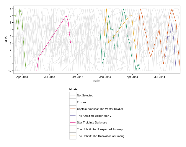
Complete. Chaos. Even if we highlight certain movies and push others to the background it’s still a bit of a mess (select the picture to see a larger/longer chart):

# set the color for all the 'background' movies
drt <- combined %>%  select(Title, rank, date) %>% mutate(color="Not Selected")

# _somewhat_ arbitrary selection here
selected_titles <- c("Frozen",
                     "Captain America: The Winter Soldier", 
                     "The Amazing Spider-Man 2", 
                     "Star Trek Into Darkness", 
                     "The Hobbit: An Unexpected Journey", 
                     "The Hobbit: The Desolation of Smaug")

# we'll use the Title field for the color factor levels
drt[drt$Title %in% selected_titles,]$color <- drt[drt$Title %in% selected_titles,]$Title
drt$color <- factor(drt$color, levels = c("Not Selected", selected_titles), ordered = TRUE)

# by using a manual color scale and our new factor variable, we can 
# highlight the few selected_titles. You'll need to use a different RColorBrewer scale
# if you up the # of movies too much, tho.

ggplot(drt, aes(x=date, y=rank, group=Title)) +
  geom_line(aes(color=color)) +
  scale_x_date(expand=c(0,0)) +
  scale_y_reverse(breaks=c(10:1)) +
  scale_color_manual(values=c("#e7e7e7", brewer.pal(length(selected_titles), "Dark2")), name="Movie") +
  theme_bw() + theme(legend.position="bottom", legend.direction="vertical", panel.grid=element_blank())

We’d have to do that interactively (via Shiny or perhaps an export to D3) to make much sense out of it.

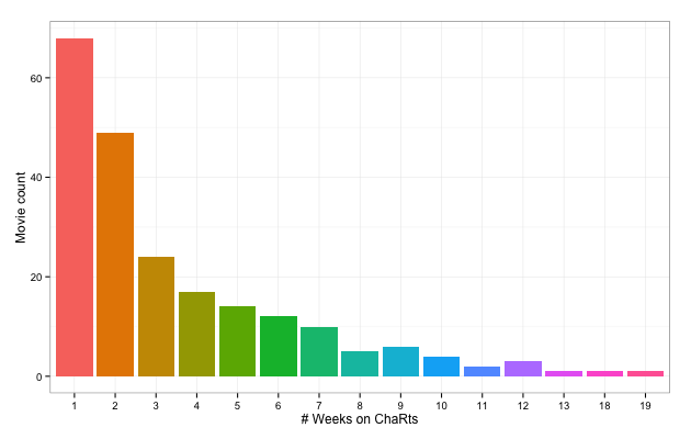
Let’s see if a “small multiples” approach gets us any further. We’ll plot each movie’s rank over time and order them by the number of weeks they were on the piRate charts. Now, there are quite a number of movies in this data set (length(unique(combined$Title)) gives me 217 for the rda on github), so first we’ll see what the distribution by # weeks on the chaRts looks like:

combined %>% select(Title, freq) %>% 
  unique %>% ggplot(aes(x=freq)) + 
  geom_histogram(aes(fill=freq)) + 
  labs(x="# Weeks on ChaRts", y="Movie count") + 
  theme_bw() + 
  theme(legend.position="none")

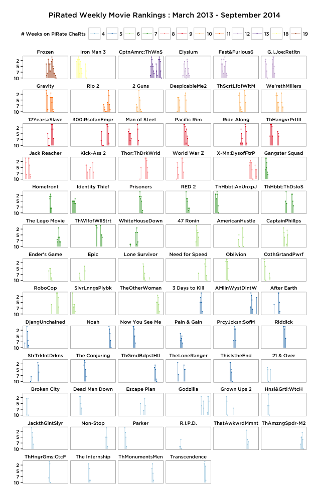
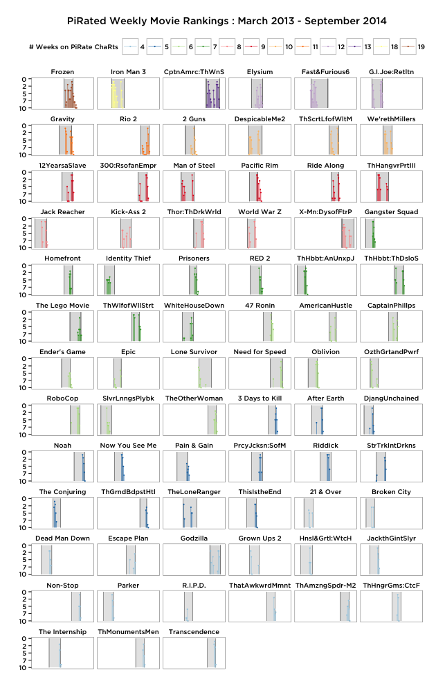
There are quite a few “one/two-hit-wonders/plunders” so we’ll make the cutoff for our facets at 4+ weeks (which also gives us just enough ColorBrewer colors to work with). Some of the movie titles are quite long, and I think it makes sense to label each facet by the movie name, so first we’ll abbreviate the names and then make the plot, coloring the facets by # of weeks on the piRate chaRts (select chart for larger version):

# abbreviate the titles
combined$short.title <- abbreviate(combined$Title, minlength=14)

# order the new short.title factor by # wks on charts
combined$short.title <- factor(combined$short.title, levels=unique(combined$short.title[order(-combined$freq)], ordered=TRUE))

gg <- ggplot(data=combined %>% filter(as.numeric(freq)>=4), aes(x=date, y=rank, group=short.title))
gg <- gg + geom_segment(aes(x=date, xend=date, y=10, yend=rank, color=freq), size=0.25)
gg <- gg + geom_point(aes(color=freq), size=1)
gg <- gg + scale_color_brewer(palette = "Paired", name="# Weeks on PiRate ChaRts")
gg <- gg + scale_fill_brewer(palette = "Paired", name="# Weeks on PiRate ChaRts")
gg <- gg + scale_y_reverse(label=floor)
gg <- gg + labs(x="", y="", title="PiRated Weekly Movie Rankings : March 2013 - September 2014")
gg <- gg + facet_wrap(~short.title, ncol=6)
gg <- gg + theme_bw()
gg <- gg + theme(text=element_text(family="Gotham Medium"))
gg <- gg + theme(strip.background=element_blank())
gg <- gg + theme(panel.grid=element_blank())
gg <- gg + theme(axis.ticks.x=element_blank())
gg <- gg + theme(axis.text.x=element_blank())
gg <- gg + theme(legend.position="top")
gg

The title of the post should make a bit more sense now as Frozen is the clear “winner” (can it be winning to be the one with the most unrealized revenue?). This visual inspection alone sheds some light on piRate habits, but we’ll need more data to confirm any nascent hypotheses.

Augmenting our PiRate Data

So far, we know movie frequency (# weeks on the chaRts) and rank over time. We could definitely use more movie metadata. Since we have the IMDb movie id from the TorrentFreak posts, we can use the Open Movie Database API (OMDb) by Brian Fritz to retrieve a great deal more information, including many details from Rotten Tomatoes. This time we use httr and jsonlite to process the API queries. The API response is clean enough to do a very quick conversion:

# call out to the OMDB API for rotten tomatoes and other bits of info
getOMDBInfo <- function(imdb.ids) {

  do.call("rbind", pblapply(unique(imdb.ids), function(imdb.id) {

    dat <- GET(sprintf("http://www.omdbapi.com/?i=%s&tomatoes=TRUE", imdb.id))
    data.frame(fromJSON(content(dat, as="text")), stringsAsFactors=FALSE)

  }))

}

# makes 10K 10000 (etc)
# adapted from http://stackoverflow.com/a/15015037/1457051
currencyToNumeric <- function(vector) {

  vector <- as.character(vector) %>% gsub("(\$|,| )", "", .) %>% as.numeric

  k_positions <- grep("K", vector, ignore.case=TRUE)
  result[k_positions] <- as.numeric(gsub("K", "", vector[k_positions])) * 1000

  m_positions <- grep("M", vector, ignore.case=TRUE)
  result[m_positions] <- as.numeric(gsub("M", "", vector[m_positions])) * 1000000

  return(result)

}

cleanUpOMDB <- function(omdb) {

  omdb$imdbVotes <- as.numeric(gsub(",", "", omdb$imdbVotes))
  omdb$tomatoUserReviews <- as.numeric(gsub(",", "", omdb$tomatoUserReviews))

  # only convert some columns to numeric

  for(col in c("Metascore", "imdbRating", "tomatoUserRating",
               "tomatoMeter", "tomatoRating", "tomatoReviews",
               "tomatoFresh", "tomatoRotten", "tomatoUserMeter")) {
    omdb[,col] <- as.numeric(omdb[,col])
  }

  omdb$BoxOffice <- currencyToNumeric(omdb$BoxOffice)

  omdb$DVD <- as.Date(omdb$DVD, format="%d %b %Y")
  omdb$Released <- as.Date(omdb$Released, format="%d %b %Y")

  omdb$Rated <- factor(omdb$Rated)
  omdb$Runtime <- as.numeric(gsub(" *min", "", omdb$Runtime))

  omdb

}

cleanUpOMDB(getOMDBInfo(combined$imdb.id))
combined <- merge(combined, omdb, by.x="imdb.id", by.y="imdbID")

Even the OMDb data needs some cleanup and conversion to proper R data types. We also convert 10m to 10000000 so we can actually use the revenue metadata. If you inspect the combined data frame, you’ll see there are missing and/or errant bits of information, even from the cleaned OMDb data. We need to fill in DVD release dates and fix the MPAA ratings for a few titles. Again, doing this programmatically (vs by hand) helps make this process usable at a later date if we need to re-scrape the data.

combined[combined$Title=="12 Years a Slave",]$DVD <- as.Date("2014-03-04")
combined[combined$Title=="Breakout",]$DVD <- as.Date("2013-09-17")
combined[combined$Title=="Dead in Tombstone",]$DVD <- as.Date("2013-10-22")
combined[combined$Title=="Dhoom: 3",]$DVD <- as.Date("2014-04-15")
combined[combined$Title=="Ender's Game",]$DVD <- as.Date("2014-02-11")
combined[combined$Title=="Epic",]$DVD <- as.Date("2013-08-20")
combined[combined$Title=="Iron Man: Rise of Technovore",]$DVD <- as.Date("2013-04-16")
combined[combined$Title=="Once Upon a Time in Mumbai Dobaara!",]$DVD <- as.Date("2013-10-26")
combined[combined$Title=="Redemption",]$DVD <- as.Date("2013-09-24")
combined[combined$Title=="Rise of the Guardians",]$DVD <- as.Date("2013-03-12")
combined[combined$Title=="Scavengers",]$DVD <- as.Date("2013-09-03")
combined[combined$Title=="Shootout at Wadala",]$DVD <- as.Date("2013-06-15")
combined[combined$Title=="Sleeping Beauty",]$DVD <- as.Date("2012-04-10")
combined[combined$Title=="Son of Batman",]$DVD <- as.Date("2014-05-06")
combined[combined$Title=="Stand Off",]$DVD <- as.Date("2013-03-26")
combined[combined$Title=="Tarzan",]$DVD <- as.Date("2014-08-05")
combined[combined$Title=="The Hangover Part III",]$DVD <- as.Date("2013-10-08")
combined[combined$Title=="The Wicked",]$DVD <- as.Date("2013-04-30")
combined[combined$Title=="Welcome to the Punch",]$DVD <- as.Date("2013-05-08")

# some ratings were missing and/or incorrect
combined[combined$Title=="Bad Country",]$Rated <- "R"
combined[combined$Title=="Breakout",]$Rated <- "R"
combined[combined$Title=="Dhoom: 3",]$Rated <- "Unrated"
combined[combined$Title=="Drive Hard",]$Rated <- "PG-13"
combined[combined$Title=="Once Upon a Time in Mumbai Dobaara!",]$Rated <- "Unrated"
combined[combined$Title=="Scavengers",]$Rated <- "PG-13"
combined[combined$Title=="Shootout at Wadala",]$Rated <- "Unrated"
combined[combined$Title=="Sleeping Beauty",]$Rated <- "Unrated"
combined[combined$Title=="Sparks",]$Rated <- "Unrated"
combined[combined$Title=="Street Fighter: Assassin's Fist",]$Rated <- "Unrated"
combined[combined$Title=="The Colony",]$Rated <- "R"
combined[combined$Title=="The Last Days on Mars",]$Rated <- "R"
combined[combined$Title=="The Physician",]$Rated <- "PG-13"

# normalize the ratings (Unrated == Not Rated)
combined[combined$Rated=="Not Rated", "Rated"] <- "Unrated"
combined$Rated <- factor(as.character(combined$Rated))

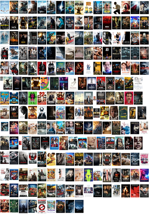
We now have quite a bit of data to try to find some reason for all this piRacy (once more, a reminder to use the github repo to reproduce this R project). We can have some fun, first, and use R (with some help from ImageMagick) to grab all the movie posters and make a montage out of them in decending order (based on # weeks on the pirate charts):

downloadPosters <- function(combined, .progress=TRUE) {

  posters <- combined %>% select(imdb.id, Poster) %>% unique

  invisible(mapply(function(id, img) {
    dest_file <- sprintf("data/posters/%s.jpg", id)
    if (!file.exists(dest_file)) {
      if (.progress) {
        message(img)
        GET(img, write_disk(dest_file), progress("down"))
      } else {
        GET(img, write_disk(dest_file))
      }
    }
  }, posters$imdb.id, posters$Poster))

}

downloadPosters(combined)

descending_ids <- combined %>% arrange(desc(freq)) %>% select(imdb.id) %>% unique %>% .$imdb.id

system(paste("montage ",
             paste(sprintf("data/posters/%s.jpg", descending_ids), collapse=" "),
             " -geometry +10+23 data/montage.png"))

system("convert data/montage.png -resize 480 data/montage.png")

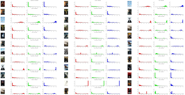
Thirty-six movies made it to “#1” in the piRate top 10 charts, lets see if there was anything common across these posters for them. We’ll plot the posters with their RGB histograms and order them by box office receipts (you’ll definitely want to grab the larger version from the pop-up image, perhaps even download it):

# get all the #1 hits & sort them by box office receipts
number_one <- combined %>% group_by(Title) %>% filter(rank==1, rating==max(rating)) %>% select(Title, short.title, imdb.id, rank, rating, BoxOffice) %>% ungroup %>% unique
number_one <- number_one[complete.cases(number_one),] %>% arrange(desc(BoxOffice))

# read in all their poster images
posters <- sapply(number_one$imdb.id, function(x) readJpeg(sprintf("data/posters/%s.jpg", x)))

# calculate the max bin count so we can normalize the histograms across RGB plots & movies
hist_max <- max(sapply(number_one$imdb.id, function(x) {
  max(hist(posters[[x]][,,1], plot=FALSE, breaks=seq(from=0, to=260, by=10))$counts,
      hist(posters[[x]][,,2], plot=FALSE, breaks=seq(from=0, to=260, by=10))$counts,
      hist(posters[[x]][,,3], plot=FALSE, breaks=seq(from=0, to=260, by=10))$counts)
}))

# plot the histograms with the poster, labeling with short title and $
n<-nrow(dat)
png("data/posters/histograms.png", width=3600, height=1800)
plot.new()
par(mar=rep(2, 4))
par(mfrow=c(n/3, 12))
for (i in 1:12) {
  for (j in 1:3) {
    plot(posters[[i*j]])
    hist(posters[[i*j]][,,1], col="red", xlab = "", ylab = "", main="", breaks=seq(from=0, to=260, by=10), ylim=c(0,hist_max))
    hist(posters[[i*j]][,,2], col="green", xlab = "", ylab = "", main=sprintf("%s - %s", dat[i*j,]$short.title, dollar(dat[i*j,]$BoxOffice)), breaks=seq(from=0, to=260, by=10), ylim=c(0,hist_max))
    hist(posters[[i*j]][,,3], col="blue", xlab = "", ylab = "", main="", breaks=seq(from=0, to=260, by=10), ylim=c(0,hist_max))
  }
}
dev.off()

A few stand out as being very different, but there aren’t many true commonalities between these sets of posters.

For reference, here’s what our data frame looks like so far:

str(combined)

## 'data.frame':    792 obs. of  40 variables:
##  $ Title            : chr  "12 Years a Slave" "12 Years a Slave" "12 Years a Slave" "12 Years a Slave" ...
##  $ imdb.id          : chr  "tt2024544" "tt2024544" "tt2024544" "tt2024544" ...
##  $ date             : Date, format: "2014-01-19" "2014-02-23" "2014-03-16" "2014-03-02" ...
##  $ movie            : chr  "12 Years a Slave" "12 Years a Slave" "12 Years a Slave" "12 Years a Slave" ...
##  $ rank             : num  7 1 3 3 10 1 7 5 10 10 ...
##  $ rating           : num  8.6 8.4 8.4 8.4 8.6 8.4 8.4 8.6 8.6 6.2 ...
##  $ Year             : chr  "2013" "2013" "2013" "2013" ...
##  $ Rated            : Factor w/ 5 levels "G","PG","PG-13",..: 4 4 4 4 4 4 4 4 4 4 ...
##  $ Released         : Date, format: "2013-11-08" "2013-11-08" "2013-11-08" "2013-11-08" ...
##  $ Runtime          : num  134 134 134 134 134 134 134 134 134 93 ...
##  $ Genre            : chr  "Biography, Drama, History" "Biography, Drama, History" "Biography, Drama, History" "Biography, Drama, History" ...
##  $ Director         : chr  "Steve McQueen" "Steve McQueen" "Steve McQueen" "Steve McQueen" ...
##  $ Writer           : chr  "John Ridley (screenplay), Solomon Northup (based on "Twelve Years a Slave" by)" "John Ridley (screenplay), Solomon Northup (based on "Twelve Years a Slave" by)" "John Ridley (screenplay), Solomon Northup (based on "Twelve Years a Slave" by)" "John Ridley (screenplay), Solomon Northup (based on "Twelve Years a Slave" by)" ...
##  $ Actors           : chr  "Chiwetel Ejiofor, Dwight Henry, Dickie Gravois, Bryan Batt" "Chiwetel Ejiofor, Dwight Henry, Dickie Gravois, Bryan Batt" "Chiwetel Ejiofor, Dwight Henry, Dickie Gravois, Bryan Batt" "Chiwetel Ejiofor, Dwight Henry, Dickie Gravois, Bryan Batt" ...
##  $ Plot             : chr  "In the antebellum United States, Solomon Northup, a free black man from upstate New York, is abducted and sold into slavery." "In the antebellum United States, Solomon Northup, a free black man from upstate New York, is abducted and sold into slavery." "In the antebellum United States, Solomon Northup, a free black man from upstate New York, is abducted and sold into slavery." "In the antebellum United States, Solomon Northup, a free black man from upstate New York, is abducted and sold into slavery." ...
##  $ Language         : chr  "English" "English" "English" "English" ...
##  $ Country          : chr  "USA, UK" "USA, UK" "USA, UK" "USA, UK" ...
##  $ Awards           : chr  "Won 3 Oscars. Another 204 wins & 192 nominations." "Won 3 Oscars. Another 204 wins & 192 nominations." "Won 3 Oscars. Another 204 wins & 192 nominations." "Won 3 Oscars. Another 204 wins & 192 nominations." ...
##  $ Poster           : chr  "http://ia.media-imdb.com/images/M/MV5BMjExMTEzODkyN15BMl5BanBnXkFtZTcwNTU4NTc4OQ@@._V1_SX300.jpg" "http://ia.media-imdb.com/images/M/MV5BMjExMTEzODkyN15BMl5BanBnXkFtZTcwNTU4NTc4OQ@@._V1_SX300.jpg" "http://ia.media-imdb.com/images/M/MV5BMjExMTEzODkyN15BMl5BanBnXkFtZTcwNTU4NTc4OQ@@._V1_SX300.jpg" "http://ia.media-imdb.com/images/M/MV5BMjExMTEzODkyN15BMl5BanBnXkFtZTcwNTU4NTc4OQ@@._V1_SX300.jpg" ...
##  $ Metascore        : num  97 97 97 97 97 97 97 97 97 44 ...
##  $ imdbRating       : num  8.2 8.2 8.2 8.2 8.2 8.2 8.2 8.2 8.2 6.2 ...
##  $ imdbVotes        : num  236225 236225 236225 236225 236225 ...
##  $ Type             : chr  "movie" "movie" "movie" "movie" ...
##  $ tomatoMeter      : num  NA NA NA NA NA NA NA NA NA 59 ...
##  $ tomatoImage      : chr  "N/A" "N/A" "N/A" "N/A" ...
##  $ tomatoRating     : num  NA NA NA NA NA NA NA NA NA 5.7 ...
##  $ tomatoReviews    : num  NA NA NA NA NA NA NA NA NA 37 ...
##  $ tomatoFresh      : num  NA NA NA NA NA NA NA NA NA 22 ...
##  $ tomatoRotten     : num  NA NA NA NA NA NA NA NA NA 15 ...
##  $ tomatoConsensus  : chr  "N/A" "N/A" "N/A" "N/A" ...
##  $ tomatoUserMeter  : num  NA NA NA NA NA NA NA NA NA 46 ...
##  $ tomatoUserRating : num  NA NA NA NA NA NA NA NA NA 3.1 ...
##  $ tomatoUserReviews: num  NA NA NA NA NA ...
##  $ DVD              : Date, format: "2014-03-04" "2014-03-04" "2014-03-04" "2014-03-04" ...
##  $ BoxOffice        : num  NA NA NA NA NA NA NA NA NA NA ...
##  $ Production       : chr  "N/A" "N/A" "N/A" "N/A" ...
##  $ Website          : chr  "N/A" "N/A" "N/A" "N/A" ...
##  $ Response         : chr  "True" "True" "True" "True" ...
##  $ short.title      : Factor w/ 217 levels "Frozen","Iron Man 3",..: 13 13 13 13 13 13 13 13 13 150 ...
##  $ freq             : Factor w/ 15 levels "1","2","3","4",..: 9 9 9 9 9 9 9 9 9 1 ...

Searching for Data TReasuRe

We don’t have a full movie corpus and we don’t even have a full piRate movie corups, just the “top 10“‘s. So, we’ll take a bit more pragmatic approach to seeing what makes for fandom in the realm of the scurvy dogs and continue our treasure hunt with some additional exploratory data analysis (EDA). Let’s see what the distributions look like for some of our new categorical and continuous variables:

# we'll be doing this again, so wrap it in a function
movieRanges <- function(movies, title="") {

  comb <- movies %>%
    select(short.title, rank, rating, Rated, Runtime, Metascore, imdbRating, imdbVotes,
           tomatoMeter, tomatoRating, tomatoReviews, tomatoFresh, tomatoRotten, BoxOffice) %>%
    group_by(short.title) %>% filter(row_number()==1) %>% ungroup

  comb$Rated <- as.numeric(comb$Rated)

  comb <- data.frame(short.title=as.character(comb$short.title), scale(comb[-1]))

  comb_melted <- comb %>% melt(id.vars=c("short.title"))

  cols <- colnames(comb)[-1]

  for(x in cols) {
    x <- as.character(x)
    y <- range(as.numeric(movies[, x]), na.rm=TRUE)
    comb_melted$variable <- gsub(x, sprintf("%sn[%s:%s]", x,
                                            prettyNum(floor(y[1]), big.mark=",", scientific=FALSE),
                                            prettyNum(floor(y[2]), big.mark=",", scientific=FALSE)),
                                            as.character(comb_melted$variable))
  }

  gg <- comb_melted %>% ggplot(aes(x=variable, y=value, group=variable, fill=variable))
  gg <- gg + geom_violin()
  gg <- gg + coord_flip()
  gg <- gg + labs(x="", y="")
  gg <- gg + theme_bw()
  gg <- gg + theme(legend.position="none")
  gg <- gg + theme(panel.grid=element_blank())
  gg <- gg + theme(panel.border=element_blank())
  gg <- gg + theme(axis.text.x=element_blank())
  gg <- gg + theme(axis.text.y=element_text(size=20))
  gg <- gg + theme(axis.ticks.x=element_blank())
  gg <- gg + theme(axis.ticks.y=element_blank())
  if (title != "") { gg <- gg + labs(title=title) }
  gg

}

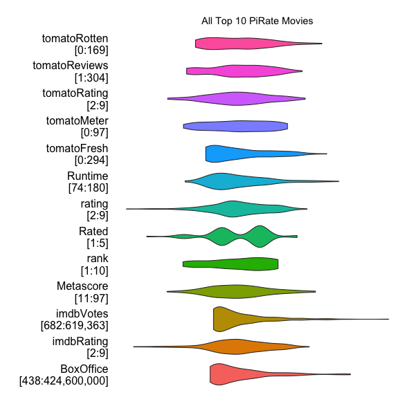
movieRanges(combined, "All Top 10 PiRate Movies")

Violin plots are mostly just prettier version of boxplots and which encode the shape of the density mass function. This orchestral view lets us compare each variable visually. IMDb votes tracks with Box Office receipts, but there are no indicators of anything truly common about these movies. It was still my belief, however, that there had to be something that got and kept these movies on the PiRate Top 10 lists.

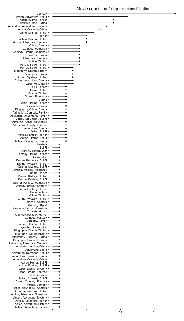
A look at movie genres does yeild some interesting findings as we see that top downloads are heavily weighted towards Comedy and Action, Adventure, Sci-Fi:

genre_table %>% arrange(desc(Count)) %>% head(10)

##                           Genre Count
## 1                        Comedy    18
## 2     Action, Adventure, Sci-Fi    11
## 3          Action, Crime, Drama     9
## 4       Action, Crime, Thriller     9
## 5  Animation, Adventure, Comedy     8
## 6         Action, Comedy, Crime     7
## 7        Crime, Drama, Thriller     6
## 8    Action, Adventure, Fantasy     5
## 9       Action, Drama, Thriller     5
## 10                       Horror     5

gg1 <- ggplot(genre_table, aes(xend=reorder(Genre, Count), yend=Count))
gg1 <- gg1 + geom_segment(aes(x=reorder(Genre, Count), y=0))
gg1 <- gg1 + geom_point(aes(x=reorder(Genre, Count), y=Count))
gg1 <- gg1 + scale_y_continuous(expand=c(0,0.5))
gg1 <- gg1 + labs(x="", y="", title="Movie counts by full genre classification")
gg1 <- gg1 + coord_flip()
gg1 <- gg1 + theme_bw()
gg1 <- gg1 + theme(panel.grid=element_blank())
gg1 <- gg1 + theme(panel.border=element_blank())
gg1

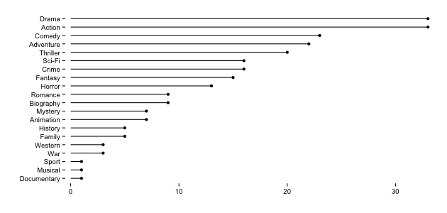
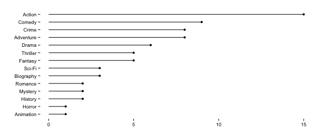
If we breakdown the full, combined genre into component parts, however, a slightly different pattern emerges:

single_genres <-  as.data.frame(table(unlist(strsplit(genre_table$Genre, ", *"))), stringsAsFactors=FALSE)
colnames(single_genres) <- c("Genre", "Count")
gg1 <- ggplot(single_genres, aes(xend=reorder(Genre, Count), yend=Count))
gg1 <- gg1 + geom_segment(aes(x=reorder(Genre, Count), y=0))
gg1 <- gg1 + geom_point(aes(x=reorder(Genre, Count), y=Count))
gg1 <- gg1 + scale_y_continuous(expand=c(0,0.5))
gg1 <- gg1 + labs(x="", y="")
gg1 <- gg1 + coord_flip()
gg1 <- gg1 + theme_bw()
gg1 <- gg1 + theme(panel.grid=element_blank())
gg1 <- gg1 + theme(panel.border=element_blank())
gg1

But, there are some commonalities between the two lists and there are definitely some genres & genre-components that rank higher, so we’ve at least got one potential indicator as to what gets you on the list. The other text fields did not yield much insight (unsurprisingly the movies gravitate towards the English language and being made in the USA), but others might have more luck.

Staying PoweR

If genre is one of the indicators that gets you on the list, what keeps you there? The presence of all the cam rips in the movie titles gave me the idea to see if there was a pattern to these movies getting into the top 10 based on date. I went back to my facet plot and decided to take a look at the movie release dates and DVD release dates by superimposing the time frames for each onto the facet graph:

gg <- ggplot(data=combined %>% filter(as.numeric(freq)>=4, !is.na(DVD)), aes(x=date, y=rank, group=short.title))
gg <- gg + geom_rect(aes(xmin=Released, xmax=DVD, ymin=0, ymax=10), fill="#dddddd", alpha=0.25)
gg <- gg + geom_segment(aes(x=Released, xend=Released, y=0, yend=10), color="#7f7f7f", size=0.125)
gg <- gg + geom_segment(aes(x=DVD, xend=DVD, y=0, yend=10), color="#7f7f7f", size=0.125)
gg <- gg + geom_segment(aes(x=date, xend=date, y=10, yend=rank, color=freq), size=0.25)
gg <- gg + geom_point(aes(color=freq), size=1)
gg <- gg + scale_color_brewer(palette = "Paired", name="# Weeks on PiRate ChaRts")
gg <- gg + scale_fill_brewer(palette = "Paired", name="# Weeks on PiRate ChaRts")
gg <- gg + scale_y_reverse(label=floor)
gg <- gg + labs(x="", y="", title="PiRated Weekly Movie Rankings : March 2013 - September 2014")
gg <- gg + facet_wrap(~short.title, ncol=6)
gg <- gg + theme_bw()
gg <- gg + theme(text=element_text(family="Gotham Medium"))
gg <- gg + theme(strip.background=element_blank())
gg <- gg + theme(panel.grid=element_blank())
gg <- gg + theme(axis.ticks.x=element_blank())
gg <- gg + theme(axis.text.x=element_blank())
gg <- gg + theme(legend.position="top")
gg

Now we’re getting somewhere. It seems that a movie hits the top charts right on opening day and continues on the charts (most of the time) until there’s a DVD release. This isn’t true for all of the movies, so let’s see which ones had longer runs than their DVD release dates (excluding ones that had only 1 extra week for post brevity):

beyond.dvd <- combined %>% 
  group_by(Title) %>% 
  summarise(n=sum(date > DVD)) %>% 
  arrange(desc(n)) %>% 
  filter(!is.na(n) & n>1)

beyond.dvd

## Source: local data frame [26 x 2]
## 
##                                Title n
## 1                        Pacific Rim 7
## 2                             Frozen 6
## 3                          Divergent 5
## 4                             2 Guns 4
## 5                            Gravity 4
## 6  The Hobbit: An Unexpected Journey 4
## 7                   12 Years a Slave 3
## 8                     3 Days to Kill 3
## 9                           47 Ronin 3
## 10                              Argo 3
## 11                      Ender's Game 3
## 12                    Now You See Me 3
## 13                          Oblivion 3
## 14                       Pain & Gain 3
## 15                             RED 2 3
## 16          The Grand Budapest Hotel 3
## 17            300: Rise of an Empire 2
## 18                    Gangster Squad 2
## 19                      Jack Reacher 2
## 20                         Prisoners 2
## 21                        Ride Along 2
## 22                   The Other Woman 2
## 23           The Wolf of Wall Street 2
## 24                   This Is the End 2
## 25              Thor: The Dark World 2
## 26                       World War Z 2

Pacific Rim was on the Top 10 PiRate ChaRts for 7 weeks past it’s DVD release date and beat Frozen O_o. Just by looking at the diversity of the titles, I’m skeptical of whether there are commonalities (beyond a desperate and cheapskate public) amongst these movies, but we’ll compare their sub-genres components (the full genre’s are almost evenly spread):

and their distributions against the previous ones (select the plot for larger version):

combined.beyond <- combined %>% group_by(Title) %>% mutate(weeks.past=sum(date>DVD)) %>% filter(date > DVD) %>% ungroup
grid.arrange(movieRanges(combined, "All Top 10 PiRate Movies"),
             movieRanges(combined.beyond, "Still in Top 10 Charts AfternPiRated AfteR DVD Release"), ncol=2)

Some ranges are tighter and we can see some movement in the MPAA ratings, but no major drivers apart from Action & Comedy.

Conclusion & Next Steps

We didn’t focus on all movies or even all piRated movies, just the ones in the TorrentFreak Top 10 list. I think adding in more diverse observations to the population would have helped identify some other key elements (besides questionalbe taste & frugality) for both what is pirated and why it may or may not land in the top 10. We did see a pretty clear pattern to the duration on the charts and some genres folks gravitate towards (though this could be due more to the fact that studios produce more of one genre than another throughout the year). It would seem from the last facet plot that Hollywood might be able to make a few more benjamins if they found some way to capitalize on the consumer’s desire to see movies in the comfort of their own abodes during the delay between theater & DVD release.

You also now have a full data set (including CSV) of metadata about pirated movies to process on your own and try to make more sense out of than I did. You can also run the script to update the data and see if anything changes with time. With the movie poster download capability, you could even analyze popularity by colors used on the posters.

We hope you had fun on this year’s piRate journey with R!

To leave a comment for the author, please follow the link and comment on his blog: Data Driven Security.

R-bloggers.com offers daily e-mail updates about R news and tutorials on topics such as: visualization (ggplot2, Boxplots, maps, animation), programming (RStudio, Sweave, LaTeX, SQL, Eclipse, git, hadoop, Web Scraping) statistics (regression, PCA, time series, trading) and more...

Pander tables inside of knitr

$
0
0

(This article was first published on rapporter, and kindly contributed to R-bloggers)
Hadley Wickham opened my eyes that calling pander to generate nifty markdown tables inside of knitr requires a special chunk option, which bothersome extra step might be saved by updating pander a bit. So it's done.

In a nutshell, whenever you call pander inside of a knitr document, instead of returning the markdown text to the standard output (as it used to happen), pander returns a knit_asis class object, which renders fine in the resulting document -- without the double comment chars, so rendering the tables in HTML, pdf or other document formats just fine.

All those who might not like the new behaviour can of course disable it via panderOptions.

Quick demo:

No need to specify `results='asis'` anymore:

```{r}
## not to split tables
panderOptions('table.split.table', Inf)
## iris still rocks
pander(head(iris))
```

But you can if you wish:

```{r}
panderOptions('knitr.auto.asis', FALSE)
pander(head(iris))
```

```{r results='asis'}
pander(head(iris))
```

Results:

No need to specify `results='asis'` anymore:


```r
## not to split tables
panderOptions('table.split.table', Inf)
## iris still rocks
pander(head(iris))
```

-------------------------------------------------------------------
Sepal.Length Sepal.Width Petal.Length Petal.Width Species
-------------- ------------- -------------- ------------- ---------
5.1 3.5 1.4 0.2 setosa

4.9 3 1.4 0.2 setosa

4.7 3.2 1.3 0.2 setosa

4.6 3.1 1.5 0.2 setosa

5 3.6 1.4 0.2 setosa

5.4 3.9 1.7 0.4 setosa
-------------------------------------------------------------------

But you can if you wish:


```r
panderOptions('knitr.auto.asis', FALSE)
pander(head(iris))
```

```
##
## -------------------------------------------------------------------
## Sepal.Length Sepal.Width Petal.Length Petal.Width Species
## -------------- ------------- -------------- ------------- ---------
## 5.1 3.5 1.4 0.2 setosa
##
## 4.9 3 1.4 0.2 setosa
##
## 4.7 3.2 1.3 0.2 setosa
##
## 4.6 3.1 1.5 0.2 setosa
##
## 5 3.6 1.4 0.2 setosa
##
## 5.4 3.9 1.7 0.4 setosa
## -------------------------------------------------------------------
```

```r
pander(head(iris))
```

-------------------------------------------------------------------
Sepal.Length Sepal.Width Petal.Length Petal.Width Species
-------------- ------------- -------------- ------------- ---------
5.1 3.5 1.4 0.2 setosa

4.9 3 1.4 0.2 setosa

4.7 3.2 1.3 0.2 setosa

4.6 3.1 1.5 0.2 setosa

5 3.6 1.4 0.2 setosa

5.4 3.9 1.7 0.4 setosa
-------------------------------------------------------------------

To leave a comment for the author, please follow the link and comment on his blog: rapporter.

R-bloggers.com offers daily e-mail updates about R news and tutorials on topics such as: visualization (ggplot2, Boxplots, maps, animation), programming (RStudio, Sweave, LaTeX, SQL, Eclipse, git, hadoop, Web Scraping) statistics (regression, PCA, time series, trading) and more...

The New Consumer Requires an Updated Market Segmentation

$
0
0

(This article was first published on Engaging Market Research, and kindly contributed to R-bloggers)
The new consumer is the old consumer with more options and fewer prohibitions. Douglas Holt calls it the postmodern market defined by differentiation: "consumer identities are being fragmented, proliferated, recombined, and turned into salable goods." It is not simply that more choices are available for learning about products, for sharing information with others and for making purchases. All that is true thanks to the internet. In addition, however, we have seen what Grant McCracken names plenitude, "an ever-increasing variety of observable ways of living and being that are continually coming into existence." Much more is available, and much more is acceptable.

For instance, the new digital consumer is no longer forced to choose one of the three major networks. Not only do they have other channels, but now they "watch" while connected through other devices. The family can get together in front of the TV with everyone doing their own thing. Shouldn't such consumer empowerment have some impact on how we segment the market?

Although we believe that the market is becoming more fragmented, our segment solutions still look the same. In fact, the most common segmentation of the digital consumer remains lifestyle. Thus, Experian's Fast Track Couple is defined by age and income with kids or likely to start a family soon. Of course, one's life stage is important and empty nesters do not behave like unmarried youths. But where is the fragmentation? What digital devices are used when and where and for what purposes? Moreover, who else is involved? We get no answers, just more of the same. For example, IBM responds to increasing diversity with its two-dimensional map based on usage type and intensity with a segment in every quadrant.


The key is to return to our new digital consumer who is doing what they want with the resources available to them. Everything may be possible but the wanting and the means impose a structure. Everyone does not own every device, nor do they use every feature. Instead, we discover recurrent patterns of specific device usage at different occasions with a limited group of others. As we have seen, the new digital consumer may own a high-definition TV, an internet-connected computer or tablet, a smartphone, a handheld or gaming console, a DVD/Blu-Ray player or recorder, a digital-media receiver for streaming, and then there is music. These devices can be for individual use or shared with others, at home or somewhere else, one at a time or multitasking, for planned activities or spontaneously, every day or for special occasions, with an owned library or online content, and the list could go on.

What can we learn from usage intensity data across such an array of devices, occasions and contexts? After all, topic modeling and sentiment analysis can be done with a "bag of words" listing the frequencies with which words occur in a text. Both are generative models assuming that the writer or speaker have something they want to say and they pick the words to express it. If all I had was a count of which words were used, could I infer the topic or the sentiment? If all I had was a measure of usage intensity across devices, occasions and contexts, could I infer something about consumer segments that would help me design or upsell products and services?

Replacing Similarity as the Basis for Clustering

Similarity, often expressed as distance, dominates cluster analysis, either pairwise distances between observations or between each observation and the segment centroids. Clusters are groupings such that observations in the same cluster are more similar to each other than they are to observations in other clusters. A few separated clouds of points on a two-dimensional plane displays the concept. However, we need lots of dimensions to describe our new digital consumer, although any one individual is likely to be close to the origin of zero intensity on all but a small subset of the dimensions. Similarity or distance loses its appeal as the number of dimensions increase and the space becomes more sparse (the curse of dimensionality).

Borrowing from topic modeling, we can use non-negative matrix factorization (NMF) without ever needing to calculate similarity. What are the topics or thematic structures underlying the usage patterns of our new digital consumer? What about personal versus shared experiences? Would we not expect a different pattern of usage behavior for those wanting their own space and those wanting to bring people together? Similarly, those seeking the "ultimate experience" within their budgets might be those with the high quality speakers or the home theater or latest gaming console and newest games. The social networker multitasks and always keeps in contact. The collector builds their library. Some need to be mobile and have access while in transit. I could continue, but hopefully it is clear that one expects to see recurring patterns in the data.

NMF uncovers those pattern by decomposing the data matrix with individuals as the rows and usage intensities as the columns. As I have shown before and show again below, the data matrix V is factored into a set of latent features forming the rows of H and individual scores on those same latent features in the rows of W. We can see the handiwork of the latent features in the repeating pattern of usage intensities. Who does A, B, C, and D with such frequency? It must be a person of this type engaging in this kind of behavior.

You can make this easy by thinking of H as a set of factor loading for behaviors (turned on its side) and W as the corresponding individual factor scores. For example, it is reasonable to believe that at least some of our new digital consumers will be gamers, so we expect to see one row of H with high weights or loadings for all the game related behaviors in the columns of H. Say that row is the first row, then the first column of W tells us how much each consumers engages in gaming activities. The higher the score in the first column of W, the more intense the gamer. People who never game get a score of zero.


In the above figure there are only two latent features. We are trying to reproduce the data matrix with as many latent features as we can interpret. To be clear, we are not trying to reproduce all the data as closely as possible because some of that data will be noise. Still, if I look at the rows of H and can quickly visualize and name all the latent features, I am a happy data analyst and will retain them all.

The number of latent features will depend on the underlying data structure and the diversity of the intensity measures. I have reported 22 latent features for a 218 item adjective rating scale. NMF, unlike the singular value decomposition (SVD) associated with factor analysis, does not attempt to capture as much variation as possible. Instead, NMF identifies additive components, and consequently we tend to see something more like micro-genre or micro-segments.

So far, I have only identified the latent features. Sometimes that is sufficient, and individuals can be classified by looking at their row in W and classifying them as belonging to the latent feature with the largest score. But what if a few of our gamers also watched live sports on TV? It is helpful to recall that latent features are shared patterns so that we would not extract a separate latent feature for gaming and for live TV sports if everyone who did one did the other, in which case there would be only one latent feature with both sets of intensity measures loading on it in H.

The latent feature scores in W can be treated like any other derived score and can enter into any other analysis as data points. Thus, we can cluster the rows of W, now that we have reduced the dimensionality from the columns of V to the columns of W and similarity has become a more meaningful metric (though care must be taken if W is sparse). The heat maps produced by the NMF package attach a dendrogram at the side displaying the results of a hierarchical cluster analysis. Given that we have the individual latent feature scores, we are free to create a biplot or cluster with any method we choose.

R Makes It So Easy with the NMF Package

Much of what you know about k-means and factor analysis generalized to NMF. That is, like factor analysis one needs to specify the number of latent features (rank r) and interpret the factor loadings contained in H (after transposing or turning it sideways). You can find all the R code and the all the output explained in a previous post. As one has the scree plot in factor analysis, there are several such plots in NMF that some believe will help one solve the number of factors problem. The NMF vignette outlines the process under the heading "Estimating the factorization rank" in Section 2.6. Personally, I find such aids to be of limited value, relying instead on interpretability as the criteria for keeping or discarding latent features.

Finally, NMF runs into all the problem experienced using k-means, the most serious being local minima. Local minima are recognized when the solution seems odd or when you repeat the same analysis and get a very different solution. Similar to k-means, one can redo the analysis many times with different random starting values. If needed, one can specify the seeding method so that a different initialization starts the iterative process (see Section 2.3 of the vignette). Adjusting the number of different random starting values until consistent solutions are achieved seems to work quite well with marketing data that contain separable groupings of rows and columns. That is, factorization works best when there are actual factors generating the data matrix, in this case, types of consumers and kinds of activities that are distinguishable (e.g., some game and some do not, some only stream and others rent or own DVDs, some only shop online and others search online but buy locally).

To leave a comment for the author, please follow the link and comment on his blog: Engaging Market Research.

R-bloggers.com offers daily e-mail updates about R news and tutorials on topics such as: visualization (ggplot2, Boxplots, maps, animation), programming (RStudio, Sweave, LaTeX, SQL, Eclipse, git, hadoop, Web Scraping) statistics (regression, PCA, time series, trading) and more...

What does CNN have in common with Carmen Reinhart, Kenneth Rogoff, and Richard Tol: They all made foolish, embarrassing errors that would never have happened had they been using R Markdown

$
0
0

(This article was first published on Statistical Modeling, Causal Inference, and Social Science » R, and kindly contributed to R-bloggers)

Rachel Cunliffe shares this delight:

scotland

Had the CNN team used an integrated statistical analysis and display system such as R Markdown, nobody would’ve needed to type in the numbers by hand, and the above embarrassment never would’ve occurred.

And CNN should be embarrassed about this: it’s much worse than a simple typo, as it indicates they don’t have control over their data. Just like those Rasmussen pollsters whose numbers add up to 108%. I sure wouldn’t hire them to do a poll for me!

I was going to follow this up by saying that Carmen Reinhart and Kenneth Rogoff and Richard Tol should learn about R Markdown—but maybe that sort of software would not be so useful to them. Without the possibility of transposing or losing entire columns of numbers, they might have a lot more difficulty finding attention-grabbing claims to publish.

Ummm . . . I better clarify this. I’m not saying that Reinhart, Rogoff, and Tol did their data errors on purpose. What I’m saying is that their cut-and-paste style of data processing enabled them to make errors which resulted in dramatic claims which were published in leading journals of economics. Had they done smooth analyses of the R Markdown variety (actually, I don’t know if R Markdown was available back in 2009 or whenever they all did their work, but you get my drift), it wouldn’t have been so easy for them to get such strong results, and maybe they would’ve been a bit less certain about their claims, which in turn would’ve been a bit less publishable.

To put it another way, sloppy data handling gives researchers yet another “degree of freedom” (to use Uri Simonsohn’s term) and biases claims to be more dramatic. Think about it. There are three options:

1. If you make no data errors, fine.

2. If you make an inadvertent data error that works against your favored hypothesis, you look at the data more carefully and you find the error, going back to the correct dataset.

3. But if you make an inadvertent data error that supports your favored hypothesis (as happened to Reinhart, Rogoff, and Tol), you have no particular motivation to check, and you just go for it.

Put these together and you get a systematic bias in favor of your hypothesis.

Science is degraded by looseness in data handling, just as it is degraded by looseness in thinking. This is one reason that I agree with Dean Baker that the Excel spreadsheet error was worth talking about and was indeed part of the bigger picture.

Reproducible research is higher-quality research.

P.S. Some commenters write that, even with Markdown or some sort of integrated data-analysis and presentation program, data errors can still arise. Sure. I’ll agree with that. But I think the three errors discussed above are all examples of cases where an interruption in the data flow caused the problem, with the clearest example being the CNN poll, where, I can only assume, the numbers were calculated using one computer program, then someone read the numbers off a screen or a sheet of paper and typed them into another computer program to create the display. This would not have happened using an integrated environment.

The post What does CNN have in common with Carmen Reinhart, Kenneth Rogoff, and Richard Tol: They all made foolish, embarrassing errors that would never have happened had they been using R Markdown appeared first on Statistical Modeling, Causal Inference, and Social Science.

To leave a comment for the author, please follow the link and comment on his blog: Statistical Modeling, Causal Inference, and Social Science » R.

R-bloggers.com offers daily e-mail updates about R news and tutorials on topics such as: visualization (ggplot2, Boxplots, maps, animation), programming (RStudio, Sweave, LaTeX, SQL, Eclipse, git, hadoop, Web Scraping) statistics (regression, PCA, time series, trading) and more...

Webinar September 25: Data Science with R

$
0
0

(This article was first published on Revolutions, and kindly contributed to R-bloggers)

A quick heads up that if you'd like to get a great introduction to doing data science with the R language, Joe Rickert will be giving a free webinar next Thursday, September 25: Data Science with R. Regular readers of the blog will be familiar with Joe's posts on this topic. A few recent examples include posts on comparing machine learning models, predictive models for airline delays, agent-based models, and many more. Register for the live webinar and Q&A with Joe, plus access to the slides and replay after the live session. Here's the overview:

Whenever data scientists are asked about what software they use R always comes up at the top of the list. In one recent survey, only SQL was rated higher than R. In this webinar we will explore what makes R so popular and useful. Starting with the big picture, we describe how R is organized and how to find your way around the R world. Then we will work through some examples highlighting features of R that make it attractive for data science work including:

  • Acquiring data
  • Data manipulation
  • Exploratory data analysis
  • Model building
  • Machine learning

Revolution Analytics webinars: Data Science with R

To leave a comment for the author, please follow the link and comment on his blog: Revolutions.

R-bloggers.com offers daily e-mail updates about R news and tutorials on topics such as: visualization (ggplot2, Boxplots, maps, animation), programming (RStudio, Sweave, LaTeX, SQL, Eclipse, git, hadoop, Web Scraping) statistics (regression, PCA, time series, trading) and more...

Yep. He made it; country voted No.

$
0
0

(This article was first published on » R, and kindly contributed to R-bloggers)

Keep Calm And Carry On Yesterday, more Scots than ever since universal suffrage was introduced cast a ballot on the matter of independence. The turnout was itself phenomenal and that implicating a series of questions for the government authorities and citizens, but for the time being the sole question was: would this benefit one side or the other? The verdict favored the "NO"--better together--by a margin little higher than indicated by major polling houses over the last week. And this returns to the point I raised roughly a month ago: the evidence from political science literature suggests that voters who failed to promptly decide are more likely to vote for the status quo in referendums like this.

Scots

To leave a comment for the author, please follow the link and comment on his blog: » R.

R-bloggers.com offers daily e-mail updates about R news and tutorials on topics such as: visualization (ggplot2, Boxplots, maps, animation), programming (RStudio, Sweave, LaTeX, SQL, Eclipse, git, hadoop, Web Scraping) statistics (regression, PCA, time series, trading) and more...

Mini-tour

$
0
0

(This article was first published on Gianluca Baio's blog, and kindly contributed to R-bloggers)
The last two days have been kind of a very interesting mini-tour for me $-$ yesterday the Symposium that we organised at UCL (the picture on the left is not a photo taken yesterday) and today the workshop on efficient methods for value of information, in Bristol.

I think we'll put the slides from yesterday's talks on the symposium website shortly. 

To leave a comment for the author, please follow the link and comment on his blog: Gianluca Baio's blog.

R-bloggers.com offers daily e-mail updates about R news and tutorials on topics such as: visualization (ggplot2, Boxplots, maps, animation), programming (RStudio, Sweave, LaTeX, SQL, Eclipse, git, hadoop, Web Scraping) statistics (regression, PCA, time series, trading) and more...

momentify R package

$
0
0

(This article was first published on Statisfaction » R, and kindly contributed to R-bloggers)

I presented today an arxived paper of my postdoc at the big success Young Bayesian Conference in Vienna. The big picture of the talk is simple: there are situations in Bayesian nonparametrics where you don’t know how to sample from the posterior distribution, but you can only compute posterior expectations (so-called marginal methods). So e.g. you cannot provide credible intervals. But sometimes all the moments of the posterior distribution are available as posterior expectations. So morally, you should be able to say more about the posterior distribution than just reporting the posterior mean. To be more specific, we consider a hazard (h) mixture model

\displaystyle h(t)=\int k(t;y)\mu(dy)

where k is a kernel, and the mixing distribution \mu is random and discrete (Bayesian nonparametric approach).

We consider the survival function S which is recovered from the hazard rate h by the transform

\displaystyle S(t)=\exp\Big(-\int_0^t h(s)ds\Big)

and some possibly censored survival data having survival S. Then it turns out that all the posterior moments of the survival curve S(t) evaluated at any time t can be computed.

The nice trick of the paper is to use the representation of a distribution in a [Jacobi polynomial] basis where the coefficients are linear combinations of the moments. So one can sample from [an approximation of] the posterior, and with a posterior sample we can do everything! Including credible intervals.

I’ve wrapped up the few lines of code in an R package called momentify (not on CRAN). With a sequence of moments of a random variable supported on [0,1] as an input, the package does two things:

  • evaluates the approximate density
  • samples from it

A package example for a mixture of beta and 2 to 7 moments gives that result:

mixture


To leave a comment for the author, please follow the link and comment on his blog: Statisfaction » R.

R-bloggers.com offers daily e-mail updates about R news and tutorials on topics such as: visualization (ggplot2, Boxplots, maps, animation), programming (RStudio, Sweave, LaTeX, SQL, Eclipse, git, hadoop, Web Scraping) statistics (regression, PCA, time series, trading) and more...

Using the Debug Option in readDICOMfile()

$
0
0

(This article was first published on Rigorous Analytics, and kindly contributed to R-bloggers)
Some recent activity in stackoverflow was brought to my attention.  Specifically, several questions were raised with reading files into R using readDICOMFile() in the oro.dicom package. The questions did highlight some inadequacies in the code, and I would like to thank the person who brought these issues to the surface.  Some of the errors that occurred were due to the fact that the files are not valid DICOM files, they were created in the early 1990s around the same time that the DICOM Standard was established. 

The result of these questions is twofold
  1. I have modified some of the code to overcome difficiencies that were highlighted.  These modifications will be available in the next release of oro.dicom (0.4.2). 
  2. I would like to raise the profile of a useful option in readDICOMFile(), the debug = TRUE input parameter.  
Let's take a closer look at "debugging" the header information in DICOM files.   The file of interest CR-MONO1-10-chest.dcm is available for download.  Note, you will have to uncompress this file before reading it.  It is not necessary to rename it with a ".dcm" extension, but it looks nicer.


The first attempt at reading this file on line #2 fails.  The error message is very informative, bytes 129-132 do not contain the characters DICM which is part of the DICOM Standard.  So... it's safe to assume that this file is not a valid DICOM file.  Delving further we turn on the debugging option (line #4) and are able to see what the first 128 bytes, which are skipped by default as part of the DICOM Standard, look like.  They obviously contain information.  By setting skipFirst128=FALSE and DICM=FALSE (line #13) we can override the default settings are start reading information from the first set of bytes.  This does the trick and with the debugging option turned on every field from the header is displayed.  No errors have occurred, so we can display the image data from this file (line #40) below. 
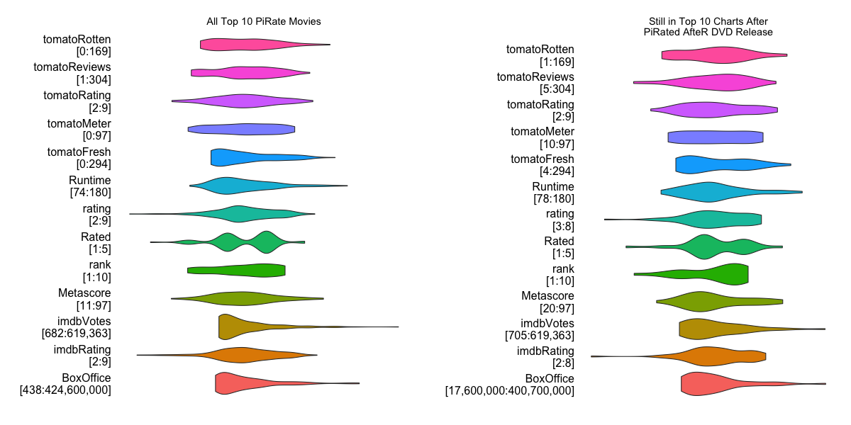
To leave a comment for the author, please follow the link and comment on his blog: Rigorous Analytics.

R-bloggers.com offers daily e-mail updates about R news and tutorials on topics such as: visualization (ggplot2, Boxplots, maps, animation), programming (RStudio, Sweave, LaTeX, SQL, Eclipse, git, hadoop, Web Scraping) statistics (regression, PCA, time series, trading) and more...

Brazilian Presidential Election

$
0
0

(This article was first published on » R, and kindly contributed to R-bloggers)

For those who follow this tale, the chart below shows the hitherto of vote intentions among the viable candidates as reported in various polls. Data collected over 2012 were simply disregarded and those from 2013 enter in the model as prior values (covariance) for the 2014 estimates. The big dots at the end of the graphs are my best guess where a particular candidate will end. The "plus" signs represent polling data estimates.

Neves (PSDB) shows a drift reaction in the last polls, in association with Marina's falling the gap between them narrows. Although this trend is not clear across all polls, one major national polling house – Ibope has picked it up with intense this week.
Perhaps most importantly, while Marina turns down, the polls suggest the government is recovering and has now the same share as in April this year. It's this trend I'd like to pay attention over the coming two weeks. If the big move in sentiment towards Marina (PSB) captured by the polls over the last weeks is genuine or ephemeral.

Finally, the undecideds are still significant in number: 8%, which means about 11 million of fellows. So, this stock of voters may play a role in the final spin of the campaign. Actually, who decide now, tend to be consistent and avoid decision costs bringing her decision to the runoff if her candidate succeed the primary.

DILMA ROUSSEFF (PT)
pt
MARINA SILVA (PSB)
psb
AÉCIO NEVES (PSDB)
psdb
OTHERS
others

To leave a comment for the author, please follow the link and comment on his blog: » R.

R-bloggers.com offers daily e-mail updates about R news and tutorials on topics such as: visualization (ggplot2, Boxplots, maps, animation), programming (RStudio, Sweave, LaTeX, SQL, Eclipse, git, hadoop, Web Scraping) statistics (regression, PCA, time series, trading) and more...
Viewing all 2417 articles
Browse latest View live